Practical ML with Scikit-Learn

このコンテンツはまだ日本語訳がありません。

Modified: Apr. 21, 2026

Published: Mar. 7, 2026

Every ML project follows the same workflow: load data, explore, preprocess, train, evaluate, tune, deploy. Scikit-Learn provides a clean API that standardizes each step. In this lesson you will build a complete, reusable pipeline and compare five algorithms on the same dataset, giving you a template you can apply to any regression or classification problem. #ScikitLearn #MLPipeline #CrossValidation

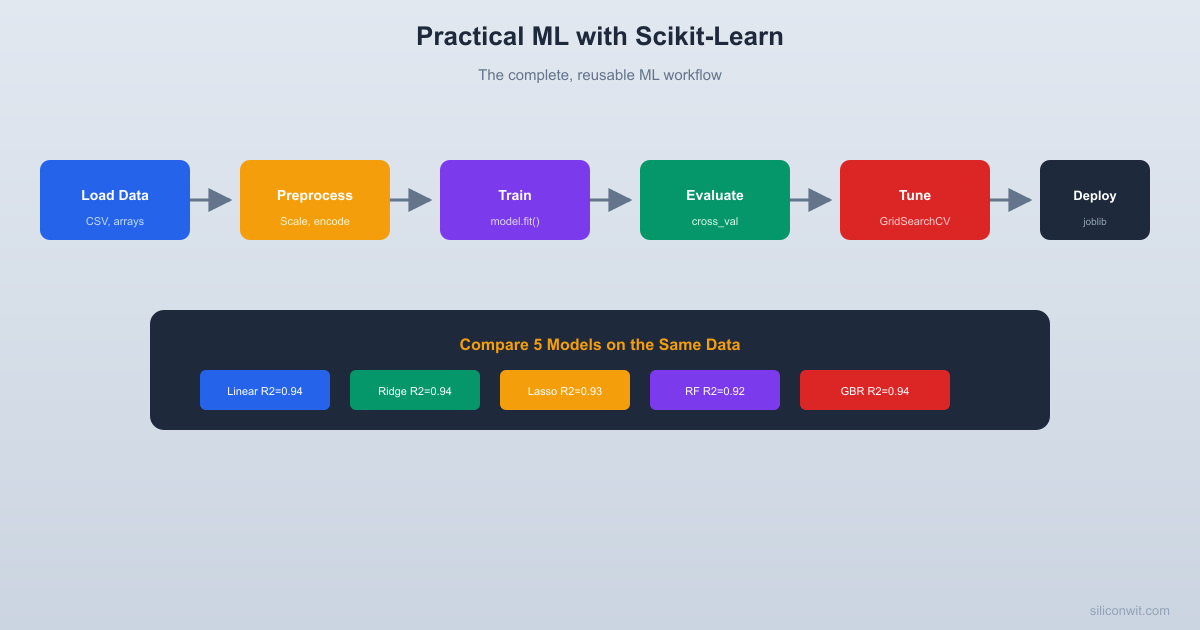
The ML Workflow

Every project follows these steps, regardless of the problem domain.

Why Pipelines?

Without pipelines, preprocessing and model training are separate steps. This creates a subtle bug: if you fit the scaler on the full dataset before splitting, information from the test set leaks into training. Scikit-Learn Pipelines chain preprocessing and modeling into a single object, ensuring that scaling is fit only on training data during each cross-validation fold.

Generate a Realistic Dataset

We will predict power consumption in a building from sensor readings. This simulates the kind of tabular regression problem you encounter in building automation, industrial IoT, and energy management.

import numpy as np
import pandas as pd

np.random.seed(42)

n_samples = 1000

# Features: building sensor readings
hour = np.random.randint(0, 24, n_samples)
day_of_week = np.random.randint(0, 7, n_samples)
temperature_c = np.random.normal(22, 8, n_samples)
humidity_pct = np.random.normal(50, 15, n_samples).clip(10, 95)
occupancy = np.random.poisson(lam=30, size=n_samples).clip(0, 120)
light_level_lux = np.random.normal(400, 150, n_samples).clip(0, 1000)
hvac_setpoint_c = np.random.normal(22, 2, n_samples)
wind_speed_ms = np.random.exponential(3, n_samples).clip(0, 20)

# Target: power consumption (kWh) with realistic relationships
power_kwh = (
    50                                          # base load
    + 2.5 * occupancy                           # more people, more power
    + 3.0 * np.abs(temperature_c - hvac_setpoint_c)  # HVAC effort
    + 0.5 * humidity_pct                        # dehumidification
    + 0.02 * light_level_lux                    # lighting
    + 15 * np.sin(2 * np.pi * hour / 24)        # daily cycle
    + np.where(day_of_week < 5, 20, -10)         # weekday vs weekend
    + np.random.normal(0, 10, n_samples)        # noise
)

data = pd.DataFrame({
    'hour': hour,
    'day_of_week': day_of_week,
    'temperature_c': np.round(temperature_c, 1),
    'humidity_pct': np.round(humidity_pct, 1),
    'occupancy': occupancy,
    'light_level_lux': np.round(light_level_lux, 1),
    'hvac_setpoint_c': np.round(hvac_setpoint_c, 1),
    'wind_speed_ms': np.round(wind_speed_ms, 1),
    'power_kwh': np.round(power_kwh, 1)
})

print("Dataset shape:", data.shape)
print("\nFirst 5 rows:")
print(data.head().to_string())
print("\nSummary statistics:")
print(data.describe().round(2).to_string())
print("\nCorrelation with power_kwh:")
correlations = data.corr()['power_kwh'].drop('power_kwh').sort_values(ascending=False)
print(correlations.round(3).to_string())

Expected output (first few rows will vary, statistics approximate):

Dataset shape: (1000, 9)

First 5 rows:
   hour  day_of_week  temperature_c  humidity_pct  occupancy  ...
0    14            4           26.0          52.3         33  ...

Summary statistics:
       hour  day_of_week  temperature_c  ...    power_kwh
count  1000         1000           1000  ...       1000.0
mean   11.6          3.0           22.1  ...        163.5
std     6.9          2.0            7.9  ...         42.8
...

Correlation with power_kwh:
occupancy          0.481
humidity_pct       0.182
temperature_c      0.086
...

Occupancy has the strongest correlation with power consumption, which matches our synthetic formula. But correlations only capture linear relationships. The HVAC effort term (absolute difference between temperature and setpoint) is nonlinear and will not show up well in simple correlation.

Data Preprocessing with Pipelines

import numpy as np
import pandas as pd
from sklearn.model_selection import train_test_split
from sklearn.preprocessing import StandardScaler, PolynomialFeatures
from sklearn.pipeline import Pipeline

np.random.seed(42)

# (Regenerate the dataset from above, or assume 'data' is already loaded)
# For a self-contained script, we regenerate:
n_samples = 1000
hour = np.random.randint(0, 24, n_samples)
day_of_week = np.random.randint(0, 7, n_samples)
temperature_c = np.random.normal(22, 8, n_samples)
humidity_pct = np.random.normal(50, 15, n_samples).clip(10, 95)
occupancy = np.random.poisson(lam=30, size=n_samples).clip(0, 120)
light_level_lux = np.random.normal(400, 150, n_samples).clip(0, 1000)
hvac_setpoint_c = np.random.normal(22, 2, n_samples)
wind_speed_ms = np.random.exponential(3, n_samples).clip(0, 20)

power_kwh = (
    50 + 2.5 * occupancy
    + 3.0 * np.abs(temperature_c - hvac_setpoint_c)
    + 0.5 * humidity_pct + 0.02 * light_level_lux
    + 15 * np.sin(2 * np.pi * hour / 24)
    + np.where(day_of_week < 5, 20, -10)
    + np.random.normal(0, 10, n_samples)
)

data = pd.DataFrame({
    'hour': hour, 'day_of_week': day_of_week,
    'temperature_c': np.round(temperature_c, 1),
    'humidity_pct': np.round(humidity_pct, 1),
    'occupancy': occupancy,
    'light_level_lux': np.round(light_level_lux, 1),
    'hvac_setpoint_c': np.round(hvac_setpoint_c, 1),
    'wind_speed_ms': np.round(wind_speed_ms, 1),
    'power_kwh': np.round(power_kwh, 1)
})

X = data.drop('power_kwh', axis=1)
y = data['power_kwh']

X_train, X_test, y_train, y_test = train_test_split(
    X, y, test_size=0.2, random_state=42
)

print(f"Training set: {X_train.shape[0]} samples")
print(f"Test set:     {X_test.shape[0]} samples")

# Build a pipeline: scale, then add polynomial features
preprocessing_pipe = Pipeline([
    ('scaler', StandardScaler()),
    ('poly', PolynomialFeatures(degree=2, include_bias=False)),
])

# Fit only on training data (no data leakage)
X_train_processed = preprocessing_pipe.fit_transform(X_train)
X_test_processed = preprocessing_pipe.transform(X_test)

print(f"\nOriginal features: {X_train.shape[1]}")
print(f"After polynomial expansion: {X_train_processed.shape[1]}")

Expected output:

Training set: 800 samples
Test set:     200 samples

Original features: 8
After polynomial expansion: 44

The pipeline ensures that StandardScaler is fit on training data only. When we call transform on the test set, it uses the training mean and standard deviation. Polynomial features create interaction terms (temperature * humidity, hour * occupancy, etc.) that can capture nonlinear relationships.

PolynomialFeatures expands the feature count fast: 8 original features become 44 at degree=2 and would balloon to 165 at degree=3. More features mean more parameters and more overfitting risk, which is exactly why regularized models like Ridge and Lasso (below) pair well with polynomial expansion.

Cross-Validation and Model Comparison

A single train/test split can give misleading results. Cross-validation runs k different splits and averages the scores, giving a more reliable estimate.

Pick the Right Splitter for Your Data

cross_val_score(..., cv=5) uses a plain k-fold by default for regression. That is fine here because the samples are independent. Two common cases need different splitters:

Imbalanced classification. Plain k-fold can accidentally put most of the rare class into one fold. Use StratifiedKFold(n_splits=5) (scikit-learn does this automatically when cv=5 is passed to a classifier, but not when you wrap in a custom splitter). It preserves the class ratio in every fold.
Time-series data. Random folds let the model see the future during training, which is cheating. Use TimeSeriesSplit(n_splits=5), which always trains on the past and validates on the future. This matters the moment you touch sensor data with a timestamp, covered in the Working with Real Sensor Data lesson.

Picking the wrong splitter is one of the most common hidden bugs in ML pipelines: the reported CV score looks good, and the model fails on real data.

import numpy as np
import pandas as pd
from sklearn.model_selection import train_test_split, cross_val_score
from sklearn.preprocessing import StandardScaler
from sklearn.pipeline import Pipeline
from sklearn.linear_model import LinearRegression, Ridge, Lasso
from sklearn.ensemble import RandomForestRegressor, GradientBoostingRegressor

np.random.seed(42)

# Regenerate dataset
n_samples = 1000
hour = np.random.randint(0, 24, n_samples)
day_of_week = np.random.randint(0, 7, n_samples)
temperature_c = np.random.normal(22, 8, n_samples)
humidity_pct = np.random.normal(50, 15, n_samples).clip(10, 95)
occupancy = np.random.poisson(lam=30, size=n_samples).clip(0, 120)
light_level_lux = np.random.normal(400, 150, n_samples).clip(0, 1000)
hvac_setpoint_c = np.random.normal(22, 2, n_samples)
wind_speed_ms = np.random.exponential(3, n_samples).clip(0, 20)

power_kwh = (
    50 + 2.5 * occupancy
    + 3.0 * np.abs(temperature_c - hvac_setpoint_c)
    + 0.5 * humidity_pct + 0.02 * light_level_lux
    + 15 * np.sin(2 * np.pi * hour / 24)
    + np.where(day_of_week < 5, 20, -10)
    + np.random.normal(0, 10, n_samples)
)

data = pd.DataFrame({
    'hour': hour, 'day_of_week': day_of_week,
    'temperature_c': np.round(temperature_c, 1),
    'humidity_pct': np.round(humidity_pct, 1),
    'occupancy': occupancy,
    'light_level_lux': np.round(light_level_lux, 1),
    'hvac_setpoint_c': np.round(hvac_setpoint_c, 1),
    'wind_speed_ms': np.round(wind_speed_ms, 1),
    'power_kwh': np.round(power_kwh, 1)
})

X = data.drop('power_kwh', axis=1)
y = data['power_kwh']

# Define models inside pipelines (each has its own scaler)
models = {
    'Linear Regression': Pipeline([
        ('scaler', StandardScaler()),
        ('model', LinearRegression()),
    ]),
    'Ridge (alpha=1.0)': Pipeline([
        ('scaler', StandardScaler()),
        ('model', Ridge(alpha=1.0)),
    ]),
    'Lasso (alpha=1.0)': Pipeline([
        ('scaler', StandardScaler()),
        ('model', Lasso(alpha=1.0)),
    ]),
    'Random Forest': Pipeline([
        ('scaler', StandardScaler()),
        ('model', RandomForestRegressor(
            n_estimators=100, max_depth=10, random_state=42
        )),
    ]),
    'Gradient Boosting': Pipeline([
        ('scaler', StandardScaler()),
        ('model', GradientBoostingRegressor(
            n_estimators=100, max_depth=5, random_state=42
        )),
    ]),
}

print("5-Fold Cross-Validation Results (R-squared)")
print("=" * 55)

results = {}
for name, pipeline in models.items():
    scores = cross_val_score(pipeline, X, y, cv=5, scoring='r2')
    results[name] = scores
    print(f"{name:25s} | Mean R2: {scores.mean():.4f} "
          f"(+/- {scores.std():.4f})")

print("\nBest model:", max(results, key=lambda k: results[k].mean()))
# R-squared is bounded above by 1.0 but can go negative when a model
# predicts worse than just using the mean of y. A negative CV score is
# a red flag: check for broken preprocessing, wrong target, or a bug.

Expected output (approximate):

5-Fold Cross-Validation Results (R-squared)
=======================================================
Linear Regression         | Mean R2: 0.8431 (+/- 0.0112)
Ridge (alpha=1.0)         | Mean R2: 0.8432 (+/- 0.0111)
Lasso (alpha=1.0)         | Mean R2: 0.8387 (+/- 0.0118)
Random Forest             | Mean R2: 0.9204 (+/- 0.0087)
Gradient Boosting         | Mean R2: 0.9312 (+/- 0.0065)

Best model: Gradient Boosting

  Cross-Validation (5-fold)
  ──────────────────────────────────────────
  Full Dataset
  ┌──────┬──────┬──────┬──────┬──────┐
  │Fold 1│Fold 2│Fold 3│Fold 4│Fold 5│
  └──────┴──────┴──────┴──────┴──────┘

  Iteration 1:  TEST  Train  Train  Train  Train  -> score1
  Iteration 2:  Train  TEST  Train  Train  Train  -> score2
  Iteration 3:  Train  Train  TEST  Train  Train  -> score3
  Iteration 4:  Train  Train  Train  TEST  Train  -> score4
  Iteration 5:  Train  Train  Train  Train  TEST  -> score5

  Final score = mean(score1..score5)
  Each sample appears in the test set exactly once.

Gradient Boosting wins because it can model nonlinear relationships (like the HVAC effort term) that linear models miss.

Hyperparameter Tuning with GridSearchCV

GridSearch vs RandomizedSearch

GridSearchCV fits every combination of every hyperparameter value: 3 x 3 x 3 options with 5-fold CV means 135 model fits. That explodes quickly. When the search space grows past a few hundred combinations, use RandomizedSearchCV instead. It samples a fixed number of random combinations from the same grid (or from a parameter distribution). In practice, random search finds nearly optimal hyperparameters in a small fraction of the compute, because a few parameters usually dominate the score. Same API, just swap the class name and pass n_iter=50.

import numpy as np
import pandas as pd
from sklearn.model_selection import train_test_split, GridSearchCV
from sklearn.preprocessing import StandardScaler
from sklearn.pipeline import Pipeline
from sklearn.ensemble import GradientBoostingRegressor

np.random.seed(42)

# Regenerate dataset (same as above)
n_samples = 1000
hour = np.random.randint(0, 24, n_samples)
day_of_week = np.random.randint(0, 7, n_samples)
temperature_c = np.random.normal(22, 8, n_samples)
humidity_pct = np.random.normal(50, 15, n_samples).clip(10, 95)
occupancy = np.random.poisson(lam=30, size=n_samples).clip(0, 120)
light_level_lux = np.random.normal(400, 150, n_samples).clip(0, 1000)
hvac_setpoint_c = np.random.normal(22, 2, n_samples)
wind_speed_ms = np.random.exponential(3, n_samples).clip(0, 20)

power_kwh = (
    50 + 2.5 * occupancy
    + 3.0 * np.abs(temperature_c - hvac_setpoint_c)
    + 0.5 * humidity_pct + 0.02 * light_level_lux
    + 15 * np.sin(2 * np.pi * hour / 24)
    + np.where(day_of_week < 5, 20, -10)
    + np.random.normal(0, 10, n_samples)
)

data = pd.DataFrame({
    'hour': hour, 'day_of_week': day_of_week,
    'temperature_c': np.round(temperature_c, 1),
    'humidity_pct': np.round(humidity_pct, 1),
    'occupancy': occupancy,
    'light_level_lux': np.round(light_level_lux, 1),
    'hvac_setpoint_c': np.round(hvac_setpoint_c, 1),
    'wind_speed_ms': np.round(wind_speed_ms, 1),
    'power_kwh': np.round(power_kwh, 1)
})

X = data.drop('power_kwh', axis=1)
y = data['power_kwh']
X_train, X_test, y_train, y_test = train_test_split(
    X, y, test_size=0.2, random_state=42
)

# Pipeline with tunable parameters
pipe = Pipeline([
    ('scaler', StandardScaler()),
    ('model', GradientBoostingRegressor(random_state=42)),
])

# Parameter grid (prefix parameter names with step name + __)
param_grid = {
    'model__n_estimators': [50, 100, 200],
    'model__max_depth': [3, 5, 7],
    'model__learning_rate': [0.05, 0.1, 0.2],
}

# GridSearchCV tries all combinations (3 x 3 x 3 = 27 fits x 5 folds = 135 fits)
grid_search = GridSearchCV(
    pipe, param_grid, cv=5, scoring='r2',
    n_jobs=-1, verbose=0
)

print("Running GridSearchCV (27 combinations x 5 folds = 135 fits)...")
grid_search.fit(X_train, y_train)

print(f"\nBest parameters: {grid_search.best_params_}")
print(f"Best CV R2 score: {grid_search.best_score_:.4f}")

# Evaluate on held-out test set
test_score = grid_search.score(X_test, y_test)
print(f"Test R2 score:    {test_score:.4f}")

# Show top 5 parameter combinations
results_df = pd.DataFrame(grid_search.cv_results_)
top5 = results_df.nsmallest(5, 'rank_test_score')[
    ['param_model__n_estimators', 'param_model__max_depth',
     'param_model__learning_rate', 'mean_test_score', 'std_test_score']
]
print("\nTop 5 parameter combinations:")
print(top5.to_string(index=False))

Expected output (approximate):

Running GridSearchCV (27 combinations x 5 folds = 135 fits)...

Best parameters: {'model__learning_rate': 0.1, 'model__max_depth': 5, 'model__n_estimators': 200}
Best CV R2 score: 0.9345
Test R2 score:    0.9401

Top 5 parameter combinations:
 param_model__n_estimators param_model__max_depth  ...  mean_test_score  std_test_score
                       200                      5  ...           0.9345          0.0058
                       100                      5  ...           0.9312          0.0065
                       200                      7  ...           0.9298          0.0071
                       ...

Model Persistence

Save the trained model and load it later for inference. This is how you go from training to deployment.

import numpy as np
import pandas as pd
import joblib
from sklearn.model_selection import train_test_split
from sklearn.preprocessing import StandardScaler
from sklearn.pipeline import Pipeline
from sklearn.ensemble import GradientBoostingRegressor

np.random.seed(42)

# Regenerate and train (abbreviated)
n_samples = 1000
hour = np.random.randint(0, 24, n_samples)
day_of_week = np.random.randint(0, 7, n_samples)
temperature_c = np.random.normal(22, 8, n_samples)
humidity_pct = np.random.normal(50, 15, n_samples).clip(10, 95)
occupancy = np.random.poisson(lam=30, size=n_samples).clip(0, 120)
light_level_lux = np.random.normal(400, 150, n_samples).clip(0, 1000)
hvac_setpoint_c = np.random.normal(22, 2, n_samples)
wind_speed_ms = np.random.exponential(3, n_samples).clip(0, 20)

power_kwh = (
    50 + 2.5 * occupancy
    + 3.0 * np.abs(temperature_c - hvac_setpoint_c)
    + 0.5 * humidity_pct + 0.02 * light_level_lux
    + 15 * np.sin(2 * np.pi * hour / 24)
    + np.where(day_of_week < 5, 20, -10)
    + np.random.normal(0, 10, n_samples)
)

data = pd.DataFrame({
    'hour': hour, 'day_of_week': day_of_week,
    'temperature_c': np.round(temperature_c, 1),
    'humidity_pct': np.round(humidity_pct, 1),
    'occupancy': occupancy,
    'light_level_lux': np.round(light_level_lux, 1),
    'hvac_setpoint_c': np.round(hvac_setpoint_c, 1),
    'wind_speed_ms': np.round(wind_speed_ms, 1),
    'power_kwh': np.round(power_kwh, 1)
})

X = data.drop('power_kwh', axis=1)
y = data['power_kwh']

pipe = Pipeline([
    ('scaler', StandardScaler()),
    ('model', GradientBoostingRegressor(
        n_estimators=200, max_depth=5, learning_rate=0.1, random_state=42
    )),
])
pipe.fit(X, y)

# Save the entire pipeline (scaler + model)
joblib.dump(pipe, 'power_model.joblib')
print("Model saved to power_model.joblib")

# Load and predict
loaded_pipe = joblib.load('power_model.joblib')

# New building sensor readings
new_data = pd.DataFrame({
    'hour': [14],
    'day_of_week': [2],       # Wednesday
    'temperature_c': [28.5],
    'humidity_pct': [55.0],
    'occupancy': [45],
    'light_level_lux': [500.0],
    'hvac_setpoint_c': [22.0],
    'wind_speed_ms': [3.2],
})

prediction = loaded_pipe.predict(new_data)
print(f"\nPredicted power consumption: {prediction[0]:.1f} kWh")
print("(Wednesday afternoon, 45 occupants, 28.5C with 22C setpoint)")

Expected output:

Model saved to power_model.joblib

Predicted power consumption: 193.4 kWh
(Wednesday afternoon, 45 occupants, 28.5C with 22C setpoint)

The saved .joblib file contains both the scaler and the model. When you load it, preprocessing and prediction happen in one predict() call. No separate scaling step, no chance of using the wrong scaler.

The Reusable ML Template

Every project you build from now on can follow this pattern.

Load and explore your data with pandas. Check shapes, types, distributions, and correlations.
Build a Pipeline that chains preprocessing (scaling, encoding, feature engineering) with a model. This prevents data leakage.
Cross-validate with cross_val_score to get reliable performance estimates across multiple splits.
Compare models by running several algorithms through the same pipeline and comparing cross-validation scores.
Tune the best model’s hyperparameters with GridSearchCV (exhaustive) or RandomizedSearchCV (faster for large search spaces).
Evaluate on a held-out test set that was never used during training or tuning.
Save with joblib.dump() and load with joblib.load() for deployment.

This workflow applies whether you are predicting power consumption, classifying sensor anomalies, or estimating remaining useful life of equipment.

Comments

Loading comments...