End-Effector Position Mapping
Sweep any joint through its full range and see how the end-effector X and Y coordinates respond. The path chart shows the actual trajectory traced in Cartesian space.
このコンテンツはまだ日本語訳がありません。
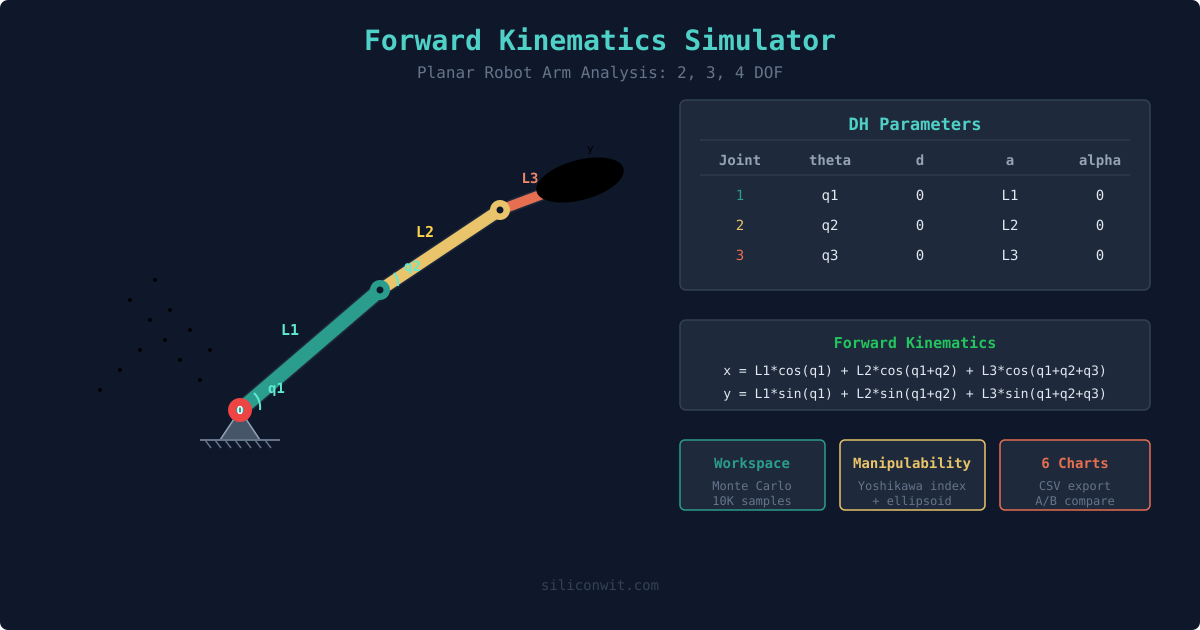
Forward kinematics answers the most fundamental question in robotics: given a set of joint angles, where is the end-effector? This simulator lets you explore that mapping for planar arms with 2, 3, or 4 degrees of freedom, while also showing the deeper structure: workspace envelopes, manipulability ellipsoids, and the Denavit-Hartenberg framework that every industrial robot controller uses. #ForwardKinematics #RobotArm #WorkspaceAnalysis
Open SimulatorEnd-Effector Position Mapping
Sweep any joint through its full range and see how the end-effector X and Y coordinates respond. The path chart shows the actual trajectory traced in Cartesian space.
Workspace Envelope
10,000 random joint configurations sampled via Monte Carlo to reveal the full reachable workspace. Points are color-coded by manipulability: green means the arm can move freely in all directions, red means it is near a singularity.
Manipulability Analysis
The Yoshikawa manipulability index and ellipsoid show how easily the arm can move at any configuration. Watch the ellipsoid collapse when the arm approaches full extension or full fold, signaling a kinematic singularity.
DH Parameters and Transforms
See the standard Denavit-Hartenberg parameter table and homogeneous transformation matrix update in real time as you move joints. This is the same framework used in industrial robot programming.
| Preset | DOF | Link Lengths (mm) | Default Angles | Use Case |
|---|---|---|---|---|
| Industrial Pick-Place | 2 | 200, 150 | 30, -45 | Simple pick-and-place reaching task |
| Drawing Robot | 3 | 120, 100, 80 | 60, -30, -20 | Pen plotter with wrist rotation |
| Flexible Manipulator | 4 | 100, 80, 60, 40 | 45, -30, 20, -15 | Highly dexterous redundant arm |
| SCARA-like | 2 | 150, 150 | 90, -90 | Equal-length arm for symmetric workspace |
For a planar N-DOF arm with revolute joints, the end-effector position is:
x = L1*cos(q1) + L2*cos(q1+q2) + ... + Ln*cos(q1+q2+...+qn)y = L1*sin(q1) + L2*sin(q1+q2) + ... + Ln*sin(q1+q2+...+qn)The Jacobian relates joint velocities to end-effector velocity: v = J * dq/dt.
The manipulability index is w = sqrt(det(J * J^T)). When w = 0, the arm is at a singularity.