Live Training Visualization
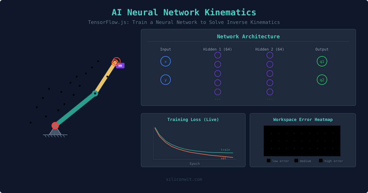
Watch the training and validation loss curves update in real time as the network trains. See whether the network is converging, plateauing, or overfitting, all in your browser.
このコンテンツはまだ日本語訳がありません。
Can a neural network learn to solve inverse kinematics? This simulator lets you find out by training a real TensorFlow.js model directly in your browser. Generate training data via motor babbling (random joint angles through forward kinematics), configure the network architecture, watch the loss curve drop in real time, then click anywhere on the workspace to compare the neural network prediction with the exact analytical solution. #NeuralNetworkIK #TensorFlowJS #MachineLearningRobotics
Open SimulatorLive Training Visualization
Watch the training and validation loss curves update in real time as the network trains. See whether the network is converging, plateauing, or overfitting, all in your browser.
Error Heatmap
After training, the workspace is color-coded by prediction error: green where the network learned well, red where it struggles. Errors are typically highest near workspace boundaries and singularities.
NN vs Analytical Comparison
Click anywhere and see both the neural network solution (purple) and analytical solution (green) simultaneously. Compare position accuracy and inference speed.
Architecture Experiments
Change the number of layers, neurons, activation function, dropout rate, and training data size. Build intuition for how network capacity and data volume affect kinematics learning.
| Preset | Samples | Layers | Neurons | Epochs | Purpose |
|---|---|---|---|---|---|
| Quick Demo | 1,000 | 1 | 32 | 50 | Fast overview, moderate accuracy |
| Standard | 5,000 | 2 | 64 | 100 | Good balance of speed and accuracy |
| High Accuracy | 20,000 | 3 | 128 | 200 | Best accuracy, longer training |
| Overfitting Demo | 200 | 3 | 128 | 300 | Demonstrates overfitting with small data |
Training data generation: The network learns by example. Random joint angles are sampled uniformly, and forward kinematics computes the corresponding end-effector positions. This creates input-output pairs: (x, y) mapped to (q1, q2).
Network architecture: A feedforward neural network with configurable hidden layers and neurons. Input: normalized (x, y) position. Output: normalized (q1, q2) joint angles. Loss function: mean squared error.
The multi-solution problem: For most targets, multiple joint configurations reach the same position (elbow-up and elbow-down). A standard feedforward network learns an average, which may not correspond to any valid configuration. This is visible in the error heatmap as regions of higher error where both solutions exist.