Lesson 1: Kinematic Joints and Constraint Analysis

A mechanism with too few degrees of freedom locks up. A mechanism with too many flops around unpredictably. The difference between a useful machine and an expensive pile of parts is whether the designer counted constraints correctly before cutting metal. The Kutzbach-Grübler equation gives you that count from the number of links and joints, and it is the first check every mechanism designer performs. In this lesson you will classify kinematic joints, calculate degrees of freedom, confront the case where the equation lies to you, and verify every answer on the same four mechanisms you can drive in our interactive simulators. #Kinematics #DOF #GrublersEquation

Learning Objectives

By the end of this lesson, you will be able to:

1. Identify different types of kinematic joints and their constraint properties
2. Calculate degrees of freedom using the Kutzbach-Grübler equation for planar mechanisms
3. Diagnose redundant constraints when the equation disagrees with physical mobility
4. Verify mechanism mobility against interactive simulators for four-bar, slider-crank, scissor-lift, and toggle-clamp mechanisms

Real-World System Problem: Modular Robotic Arm Assembly System

Consider a manufacturing facility that needs flexible automation: one day assembling electronic components, the next day handling automotive parts, and later packaging consumer goods. Traditional fixed robotic systems cannot adapt to this variety of tasks. The solution? Modular robotic arms with interchangeable joint modules that can be reconfigured for different applications. But reconfiguring blindly is dangerous: add the wrong joint and the arm either jams solid or wobbles with motions no motor controls.

System Challenge: Joint Selection for Reconfigurable Robots

Critical Engineering Questions:

• How many joints do we need for a specific task?
• Which joint types provide the required motion?
• How do we guarantee the mechanism has exactly the mobility we intend, no more and no less?
• What constraints do different joints impose on the system?

Modular Robot Design Challenge

Design Goal: Create a joint library where engineers can select and combine different joint types to build task-specific robotic arms and machines.

Key Requirements:

• Flexibility: Support various motion requirements
• Analyzability: Predict system behavior before assembly
• Optimization: Minimize complexity while maximizing capability
• Standardization: Compatible joint interfaces for easy reconfiguration

Engineering Question: Given any arrangement of links and joints, how do we predict whether it will move, how many motors it needs, and whether our prediction can be trusted?

Why Constraint Analysis Matters

Consequences of getting the count wrong:

• Lock-up when too many constraints leave zero mobility (a structure where you wanted a mechanism)
• Uncontrolled motion when too few constraints leave degrees of freedom no actuator commands
• Binding and broken parts in over-constrained assemblies that only fit because of manufacturing slop
• Wasted cost from motors and controllers driving freedoms the task never needed

Benefits of systematic analysis:

• Predictable mobility before any hardware is built
• Correct actuator count (one independent input per degree of freedom)
• Early detection of over-constraint and singular configurations
• A shared language that scales from a door hinge to a six-axis robot

Fundamental Theory: Kinematic Joints and Constraints

To solve our modular robot challenge, we need to understand how joints work and how they constrain motion.

What are Kinematic Joints?

Joint Definition

A kinematic joint (or kinematic pair) is a mechanical connection that:

• Connects two rigid bodies (links)
• Allows specific types of relative motion
• Constrains unwanted motions
• Transmits forces and moments between bodies

Key Concept: Every joint both enables desired motion and removes undesired motion. The motions it permits are its degrees of freedom; the motions it blocks are its constraints. In a plane, permitted + constrained = 3 for every joint.

In a plane, a single free body has exactly three degrees of freedom: it can translate in X, translate in Y, and rotate about the axis perpendicular to the plane. Every planar joint we attach removes some of these three freedoms. A joint that removes two freedoms (leaving one) is called a lower pair; a joint that removes only one (leaving two) is a higher pair. This single accounting rule, three freedoms minus the constraints, is the entire foundation of mobility analysis.

Classification of Planar Kinematic Joints

• Revolute Joint (R)
• Prismatic Joint (P)
• Higher Pair (Half Joint)

Revolute (Pin) Joint

Motion Allowed: Rotation about the axis perpendicular to the plane Motion Constrained: Translation in both in-plane directions Degrees of Freedom: 1   |   Constraints: 2

Planar motion	Permitted?
X-translation	❌
Y-translation	❌
Z-rotation	✅

This is a lower pair (surface contact, 2 constraints).

Applications: Robot shoulder and elbow joints, door hinges, motor shaft connections, every pin in a four-bar linkage.

Degrees of Freedom Fundamentals

Degrees of Freedom in the Plane

A free rigid body in a plane has 3 DOF:

• X-translation
• Y-translation
• Z-rotation (about the axis perpendicular to the plane)

For a mechanism of links, one link is the fixed ground, so the moving bodies contribute unconstrained freedoms before any joint is added. Joints then subtract constraints.

The Kutzbach-Grübler Equation

Kutzbach-Grübler Equation for Planar Mechanisms

Where:

• = total number of links, including the ground/frame
• = number of lower pairs (revolute or prismatic, each removing 2 constraints)
• = number of higher pairs (cam or gear contact, each removing 1 constraint)

Reading the equation: is the total freedom of all moving links; is the total constraint imposed by all joints. Mobility is what is left over.

Systematic Joint Analysis Process

1. Identify all links, and include the ground/frame as one link.

2. Classify every joint as a lower pair () or higher pair (), and confirm the constraint count.

3. Apply the Kutzbach-Grübler equation to compute the mobility.

4. Verify physically: does the predicted mobility match how the real mechanism moves? One actuator should be needed per degree of freedom.

5. Check for special cases: redundant constraints, passive joints, and singular configurations can all make the raw equation disagree with reality.

Application 1: Four-Bar Linkage (The Workhorse of Planar Mechanisms)

The four-bar linkage is the most widely used closed-chain mechanism in engineering, from windshield wipers to suspension systems to robotic grippers. We will analyze its mobility, then drive it in the simulator to confirm a single input controls the entire chain.

Simulator and hands-on lab

Open the Four-Bar Linkage Simulator

Hands-on lab: Practice with this mechanism in the Four-Bar Linkage Experiments lab. Experiment 1 (the Grashof condition) is a natural starting point for confirming that a single crank input drives the whole linkage.

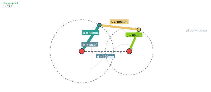
Equivalent System Model

Given the four links:

• Link 1: ground/frame (the fixed bar of length )
• Link 2: crank (input link of length )
• Link 3: coupler (floating link of length )
• Link 4: follower/rocker (output link of length )

The four joints are all pin (revolute) connections: ground-crank (), crank-coupler (), coupler-follower (), follower-ground ().

Step 1: Count Links and Joints

Click to reveal the link and joint inventory

1. Count links (include ground):

   ✅

2. Classify the joints:

   All four connections are pin joints, so they are revolute lower pairs:

   ✅

Step 2: Apply the Kutzbach-Grübler Equation

Click to reveal the mobility calculation

1. Substitute into the equation:

   ✅

   ✅

2. Interpret the result:

   • The linkage has mobility 1: a single input fully determines every link’s position.
   • Motors required: 1, applied at the crank ().
   • With one input fixed, the coupler and follower angles are completely determined by the geometry (you solve for them explicitly in the position analysis). ✅

Step 3: Verify in the Simulator

Click to reveal the simulator verification

1. Open the Four-Bar Linkage Simulator (short link siwit.co/FBL) and load the Crank-Rocker (Grashof) preset, or set , , , mm. ✅

2. Observe the single input: the simulator exposes exactly one driving variable, the crank angle. Sweep it from 0 to 360 degrees. ✅

3. Confirm mobility = 1: every other quantity the simulator plots (, , , , the coupler-point path) is fully determined by that one crank angle. There is no second freedom to set. ✅

4. Connect to the equation: the fact that one slider controls the whole figure is the physical meaning of . If the linkage had 2 DOF, the simulator would need two independent inputs to pin down the configuration. ✅

Application 2: Slider-Crank Mechanism (Replacing a Pin with a Slider)

The slider-crank converts rotation into straight-line motion and is the heart of every piston engine, pump, and compressor. It looks different from the four-bar, but its mobility is identical, and seeing why deepens the joint-counting intuition.

Simulator and hands-on lab

Open the Crank-Slider Simulator

Hands-on lab: Practice with this mechanism in the Crank-Slider Experiments lab. Experiment 1 (the baseline kinematic profile) lets you drive the single crank input and watch the piston motion it fully determines.

Equivalent System Model

The four links:

• Link 1: engine block / frame (ground)
• Link 2: crank (input)
• Link 3: connecting rod (coupler)
• Link 4: piston / slider (output)

The four joints:

• 3 revolute joints: crank-frame (), crank-rod, rod-piston
• 1 prismatic joint: piston sliding in the cylinder bore

Step 1: Count Links and Joints

Click to reveal the link and joint inventory

1. Count links (include ground):

   ✅

2. Classify the joints:

   Three pin joints plus one sliding joint, all lower pairs:

   ✅

   Note: a prismatic joint is a lower pair just like a revolute joint. Both remove 2 planar constraints, so both count toward .

Step 2: Apply the Kutzbach-Grübler Equation

Click to reveal the mobility calculation

1. Substitute:

   ✅

2. Compare to the four-bar: identical mobility. The only change from Application 1 is that one revolute joint was replaced by a prismatic joint, and since both are lower pairs with 2 constraints each, the count is unchanged. ✅

Step 3: The “Revolute at Infinity” Insight and Simulator Check

Click to reveal the geometric interpretation and verification

1. A slider is a pin on an infinitely long link. Imagine the rocker of the four-bar growing longer and longer. Its tip traces an ever-flatter arc until, in the limit, the arc becomes a straight line and the pin becomes a slider. The slider-crank is the four-bar with its follower stretched to infinity, which is why the mobility is preserved. ✅

2. Open the Crank-Slider Mechanism Simulator (short link siwit.co/CSM) and set , , . ✅

3. Confirm mobility = 1: the only driving input is the crank angle. The piston displacement, velocity, and acceleration the simulator plots are all consequences of that single input. ✅

4. Try the offset: set . The motion becomes asymmetric (the quick-return effect), but the mobility is still 1: changing geometry never changes the joint count, only the path traced. ✅

Application 3: Scissor Lift (When the Equation Lies: Grübler’s Paradox)

So far the equation has matched reality perfectly. Now we meet the case every engineer must recognize: a mechanism that moves with one degree of freedom, yet whose raw Kutzbach-Grübler count comes out negative. The scissor lift is the classic example, and resolving the contradiction is one of the most important skills in this lesson.

Simulator and hands-on lab

Open the Scissor Lift Simulator

Hands-on lab: Practice with this mechanism in the Scissor Lift Experiments lab. Experiment 1 (the baseline height and force profile) lets you raise the platform on a single actuator input and observe that it stays horizontal throughout.

Equivalent System Model

The four links:

• Link 1: base (ground)
• Link 2: arm A
• Link 3: arm B
• Link 4: platform

The five joints:

• Center pivot: revolute joint where arms A and B cross
• Arm A to base: revolute (pinned)
• Arm B to base: prismatic (rolls/slides along the base)
• Arm A to platform: prismatic (rolls/slides along the platform)
• Arm B to platform: revolute (pinned)

So: 3 revolute + 2 prismatic = 5 lower pairs.

Step 1: Apply the Equation Naively

Click to reveal the raw mobility calculation

1. Inventory:

   ✅

2. Substitute:

   ⚠️ ✅

3. Read the result literally: predicts an over-constrained structure that should not move at all, and might even bind. ✅

Step 2: Compare with Physical Reality

Click to reveal the contradiction

1. A real scissor lift clearly moves. A single hydraulic cylinder raises and lowers the platform, and the platform stays horizontal throughout. That is the behavior of a 1-DOF mechanism, not a -DOF structure. ✅

2. The contradiction:

   The equation is off by 2. This discrepancy is Grübler’s paradox. ✅

Step 3: Reconcile with Redundant Constraints

Click to reveal the resolution

1. The fix: redundant constraints. The Kutzbach-Grübler equation assumes every joint imposes independent constraints. The scissor lift’s special symmetry violates that assumption: equal-length arms pivoting at their shared midpoint force the platform to stay parallel to the base. That “stay parallel” condition is enforced more than once by the symmetric geometry, so some constraints overlap and do no new work. ✅

2. Account for the overlap. Let be the number of redundant constraints. The corrected mobility is:

   ✅

   Solving with the observed mobility:

   ✅

3. Physical source of the 2 redundancies: both prismatic joints have parallel axes and the arms are symmetric, so the orientation of the platform is pinned down by several joints that all say the same thing. Two of those constraint equations are linearly dependent on the others, so they remove no additional freedom. ✅

Step 4: Verify in the Simulator

Click to reveal the simulator verification

1. Open the Scissor Lift Mechanism Simulator (short link siwit.co/SLM). ✅

2. Confirm a single input: the simulator drives the lift with exactly one variable (the actuator length, or equivalently the scissor angle ). One input, one degree of freedom. ✅

3. Confirm the platform stays horizontal at every height. That preserved horizontal orientation is the visible signature of the redundant constraints: the symmetry enforces it automatically, which is why the raw equation over-counted the constraints. ✅

4. Conclusion: observed mobility = 1, matching the corrected calculation, not the raw . ✅

Application 4: Toggle Clamp (Mobility vs. the Singular Configuration)

A toggle clamp holds a workpiece with enormous force from a light hand effort, and stays clamped even when you let go. It is a 1-DOF four-bar, yet at one special position it behaves dramatically differently. Distinguishing the mechanism’s overall mobility from its instantaneous behavior at a singularity is the final concept of this lesson.

Simulator and hands-on lab

Open the Toggle Clamp Simulator

Hands-on lab: Practice with this mechanism in the Toggle Clamp Experiments lab. Experiment 1 (top-dead-centre and self-locking) maps directly onto the singular configuration discussed here.

Equivalent System Model

The four links:

• Link 1: clamp base (ground)
• Link 2: handle (input)
• Link 3: main link (coupler)
• Link 4: clamp arm carrying the pad (output)

The four joints: all revolute pins: handle-base (), handle-main link (), main link-clamp arm (), clamp arm-base ().

This is the same topology as the four-bar in Application 1.

Step 1: Confirm Mobility

Click to reveal the mobility calculation

1. Inventory:

   ✅

2. Substitute:

   ✅

3. Interpretation: the toggle clamp is a four-bar linkage. One input (the handle) determines the whole configuration, exactly as in Application 1. ✅

Step 2: What Happens at Top-Dead-Center

Click to reveal the singular-configuration analysis

1. The toggle (over-center) position: the clamp reaches a configuration where the handle link and main link become collinear (top-dead-center). At that instant the input crank can move while the output pad barely moves at all. ✅

2. What changes, and what does not:

   • The mobility stays 1. The mechanism still has exactly one degree of freedom; you have not added or removed any joint.
   • The instantaneous velocity ratio between input and output goes to zero (the output is momentarily stationary with respect to the input). This makes the mechanical advantage spike toward infinity: a small handle force produces a very large clamping force. ✅

3. Self-locking: because the geometry sits slightly past top-dead-center at rest, any reaction force from the clamped part tries to push the linkage back through the collinear position, where the mechanical advantage works against it. The clamp holds with no continued handle effort. This is a geometric (singular) property of one configuration, not a property of the degree-of-freedom count. ✅

Step 3: Verify in the Simulator

Click to reveal the simulator verification

1. Open the Toggle Clamp Mechanism Simulator (short link siwit.co/TCM). ✅

2. Confirm a single input: the handle angle is the only driver. One input, one degree of freedom, just as the equation says. ✅

3. Drive the handle toward top-dead-center and watch the mechanical-advantage and transmission-angle plots: mechanical advantage rises sharply as the links approach collinear, even though the mechanism never gained a degree of freedom. ✅

4. Conclusion: mobility is constant at 1 across the entire motion; the dramatic force amplification is an instantaneous singular effect of geometry. ✅

Design Application: Modular Serial Robot Arm

The four mechanisms above are closed chains (their links form loops). The modular robot arm from our opening challenge is an open chain (a series of links ending in a free end-effector), and open chains follow a simpler rule: degrees of freedom add up. Let us size the modular arm.

Open-Chain Rule: Series Joints Add

Why Serial Joints Add Their DOF

In an open serial chain with only single-DOF joints, the Kutzbach-Grübler equation reduces to a simple sum. For single-DOF joints in series:

(since an -joint open chain has links). Each serial joint adds exactly one degree of freedom, which is why robot arms are described by their joint count: a “6-axis” robot has 6 DOF.

• 2-DOF Arm
• 3-DOF Arm
• Hybrid R-R-P Arm
• 6-DOF Industrial Arm

Configuration: ground + upper arm + forearm, joined by 2 revolute joints (shoulder, elbow).

✅

Capability: positions the end-effector anywhere in its planar workspace. Needs 2 motors.

Design Guidelines for Joint Selection

DOF Optimization Strategy

1. Analyze the task first. Identify the required end-effector motions and the minimum DOF that achieves them.

2. Right-size the mobility. Avoid over-constraint (DOF , binding) and avoid unnecessary freedoms (each one costs a motor and a controller). Target DOF = task requirement, adding redundancy only when fault tolerance or obstacle avoidance justifies it.

3. Plan one actuator per degree of freedom. Input count must equal DOF for full control.

4. Verify before building. Compute mobility with Kutzbach-Grübler, then confirm against a simulation, especially for any symmetric or parallel-motion mechanism where redundant constraints may hide.

Summary and Next Steps

Key Concepts Mastered

1. Joint types: revolute and prismatic are lower pairs (1 DOF, 2 constraints); cam/gear contacts are higher pairs (2 DOF, 1 constraint).
2. Kutzbach-Grübler equation: for any planar mechanism.
3. Grübler’s paradox: redundant constraints from special geometry can make the raw count too low; the scissor lift moves with 1 DOF despite a raw count of .
4. Mobility vs. singularity: a mechanism’s DOF is global; self-locking and force spikes (the toggle clamp) are instantaneous geometric effects that do not change the DOF.
5. Open vs. closed chains: serial joints add DOF; closed loops constrain it.

The Four Mechanisms at a Glance

Mechanism				Raw DOF	Actual DOF	Simulator
Four-bar linkage	4	4	0	1	1	siwit.co/FBL
Slider-crank	4	4	0	1	1	siwit.co/CSM
Scissor lift	4	5	0	−1	1 (2 redundant)	siwit.co/SLM
Toggle clamp	4	4	0	1	1	siwit.co/TCM

Professional Design Principles

Real-World Applications

This joint-and-constraint methodology underpins:

• Industrial robots: automotive assembly, welding, painting
• Manufacturing equipment: scissor lifts, toggle-clamp fixtures, indexing tables
• Automotive systems: suspension linkages, steering mechanisms, engine slider-cranks
• Service and mobile platforms: lifts, grippers, inspection arms

Next, Position Analysis of Planar Linkages takes the four-bar linkage whose mobility we just confirmed and solves for the exact position of every link using vector loop equations, the foundation for the velocity, acceleration, and force analysis that follows.

Comments

Loading comments...