Foundation for everything
Velocity is the time derivative of position; acceleration is the derivative of velocity. You cannot find either until the positions are solved.
Mobility analysis confirmed that the four-bar linkage, slider-crank, scissor lift, and toggle clamp each move with a single degree of freedom. That tells you one input controls them, but not where that input puts the output. Turn the crank of a four-bar by a known angle and the coupler and follower take up specific angles that the geometry alone decides. Position analysis finds those angles. It is the problem you must solve before any velocity, acceleration, or force analysis, because all of those are built on top of the positions. In this lesson you write the vector loop equation for each mechanism and solve it in closed form, then check the answer in the simulator. #PositionAnalysis #VectorLoops #Freudenstein
By the end of this lesson, you will be able to:
A windshield wiper must sweep a precise arc and stop short of the A-pillar. An engine piston must reach top-dead-center exactly when the crank does. A scissor-lift platform must reach a target height and stay level. In every case the designer commits to link lengths and then has to predict, before any metal is cut, exactly where the output sits for every input position. Guessing is not an option, because a few millimetres of error can mean a wiper that hits the trim or a piston that collides with a valve.
Position analysis answers one question for a single-degree-of-freedom mechanism:
Engineering Question: Given the input link angle, what are the angles and coordinates of every other link?
For an open serial chain (a robot arm), this is direct: add the links nose to tail. For a closed chain (the four mechanisms of this course), the links form a loop that must close on itself, and that closure condition is what we solve.
Foundation for everything
Velocity is the time derivative of position; acceleration is the derivative of velocity. You cannot find either until the positions are solved.
Reachability and interference
Position analysis shows whether the output reaches its target and whether links collide or bind anywhere in the range of motion.
Path generation
A point on the coupler traces a curve. Position analysis predicts that curve, which is how linkages are made to follow a required path.
Limit positions
It locates the extreme positions where the output reverses, the basis of dead-center clamping and stroke limits.
Position, velocity, and acceleration are solved by two core methods, graphical and analytical, that you then confirm with a simulator. One further trick, the instantaneous center, is worth knowing as a quick velocity shortcut, but the course does not build on it (the fourth card explains why). These are not rivals: each answers the same question in a different way, so you use them to check one another. The three analysis lessons (this one, velocity, and acceleration) apply the same set to the same mechanisms, so it is worth meeting them together before diving into the algebra.
Graphical (drawing-instrument) method
Core method. Draw the mechanism to scale on paper and read the answer straight off the drawing. Position comes from striking arcs with a compass; velocity and acceleration come from polygons built with a set square and measured with a scale rule and protractor: the classical draughtsman’s drawing set. It is intuitive and always works, but it handles one instant at a time and only to drawing-board precision (a few percent).
Analytical (vector-loop) method
Core method. Write the loop-closure condition
Simulator (confirm and lab)
How you confirm. The interactive simulators in this course (and packages like MATLAB or 2D-linkage software) solve the loop numerically and animate the whole cycle. Every worked example ends by reading the same answer off the simulator, and the hands-on labs are built on it. It is only as trustworthy as the model you set up, so it confirms the two methods above rather than replacing them.
Instantaneous centers (worth knowing)
A velocity shortcut, not our main road. Locate the point each link instantaneously turns about (using Kennedy’s theorem) and read a velocity ratio directly, with no equations. It is a neat one-step check, but it gives velocities only: there is no instantaneous center for acceleration, so it cannot follow a problem through the full position, velocity, acceleration chain the way the graphical polygon can. We note it and use it as a check; we build on the polygon, the loop, and the simulator.
Treat them as a sequence, not a menu: draw, solve, simulate. Draw it first with the drawing set to see the mechanism and get a quick answer at the instant of interest. Solve it analytically to turn that sketch into an exact number and, crucially, to sweep the whole cycle instead of one pose. Simulate it to animate the motion, plot a full revolution, confirm the drawing and the algebra, and drive the lab exercises. The instantaneous center sits outside this sequence as an optional one-step check on a velocity ratio, nothing more.
The real payoff is cross-checking. The length you measure off a velocity polygon should equal the value you compute by differentiating the loop, which should match what the simulator reports. When all three agree, you can trust the result; when they disagree, one of them has exposed a mistake. Every worked example in these three lessons follows this rhythm, so you build the habit of confirming a kinematic answer three independent ways.
You draw a polygon, measure
| Source of error | Typical size | How to reduce it |
|---|---|---|
| Scale rule reading | choose a scale that fills the page | |
| Protractor reading | construct perpendiculars with a set square, not a protractor | |
| Compass slip | sharp lead, re-check the opening against the rule | |
| Line thickness | 0.3 mm pencil, hard grade | |
| Near-tangent intersection | unbounded | re-draw at a different instant |
| Combined, carefully drawn | 1 to 2 percent | |
| Combined, hurried | 5 to 10 percent |
The drawing is not just a warm-up for the algebra. It catches what algebra hides: a wrongly signed
Vector Loop Principle
Treat each link as a vector pointing from one joint to the next. In any closed kinematic loop, walking around the links and back to the start gives zero net displacement:
This single geometric fact turns a drawing into algebra. Each vector contributes a cosine term to the x-equation and a sine term to the y-equation, giving two scalar equations per loop.
The power of the method is that it is the same for every linkage. You label the links as vectors, write the loop sum, split it into x and y components, mark which angles are known and which are unknown, and solve. The four-bar gives two equations in two unknown angles. The slider-crank gives two equations in one unknown angle and one unknown distance. The procedure never changes; only the bookkeeping does.
We use the same link labels as the simulator: link
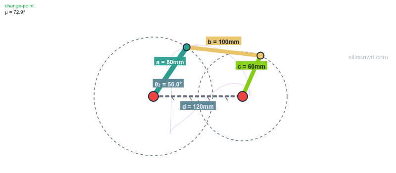
Four-Bar Vector Loop
X-component:
Y-component:
Known: link lengths
These are two nonlinear equations in two unknowns. The next section solves them in closed form, so no guessing or iteration is needed.
This is the central worked example of the lesson. We solve the four-bar position problem exactly, then read the same angles off the simulator.
Simulator and hands-on lab
Hands-on lab: Continue in the Four-Bar Linkage Experiments lab. Experiment 5 (coupler-curve exploration) extends the position analysis below to the path traced by a coupler point.
The graphical method solves the position problem with the drawing set alone, no equations. It is the fastest way to see the answer, and it doubles as a check on the algebra that follows. The whole trick is that two of the four link lengths (
Choose and note a scale. Pick a length scale that fills the page, say 1 cm = 20 mm, and write it on the drawing. Every length below is laid off with the scale rule at this scale. ✅
Ground and crank. Draw the ground
Intersect the coupler and follower arcs. Open the compass to the coupler length
Measure the unknowns. Draw

The drawing gives each angle to within a degree or so. The closed-form Freudenstein solution below pins them to
Isolate the coupler terms in both component equations:
Square both equations and add. Because
Divide through by
Define the three constants from the link lengths only:
Evaluate for
Expand
Evaluate at
Solve the quadratic. The two roots give the two assembly modes:
Open mode (minus sign):
The crossed mode (plus sign) gives the other branch, discussed in Step 5.
Eliminate
Quadratic coefficients:
Solve (open mode, minus sign):
Substitute back into the original loop equation. This is the mandatory last step of every position solution, not a flourish (
Both residuals should come out to a fraction of a millimetre against link lengths of tens of millimetres. If either is a few millimetres or more, something is wrong: most often a mismatched assembly mode, an angle left in degrees where radians were needed, or a sign slip in a quadratic coefficient. The loop either closes or it does not, and this check takes fifteen seconds. Make it a habit now and it will save an entire question later. ✅
Repeat the solution for crank angles across a full turn (open mode). A short Python script automates it: ✅
import numpy as np
def four_bar_position(a, b, c, d, theta2_deg, mode="open"):    """Closed-form four-bar position. a=crank, b=coupler, c=follower, d=ground."""    t2 = np.radians(theta2_deg)    K1, K2 = d/a, d/c    K3 = (a**2 - b**2 + c**2 + d**2) / (2*a*c)    A = np.cos(t2) - K1 - K2*np.cos(t2) + K3    B = -2*np.sin(t2)    C = K1 - (K2 + 1)*np.cos(t2) + K3    s = -1 if mode == "open" else 1    t4 = 2*np.arctan2(-B + s*np.sqrt(B**2 - 4*A*C), 2*A)
    K4 = d/b    K5 = (c**2 - d**2 - a**2 - b**2) / (2*a*b)    D = np.cos(t2) - K1 + K4*np.cos(t2) + K5    E = -2*np.sin(t2)    F = K1 + (K4 - 1)*np.cos(t2) + K5    t3 = 2*np.arctan2(-E + s*np.sqrt(E**2 - 4*D*F), 2*D)    return np.degrees(t3) % 360, np.degrees(t4) % 360
for th2 in range(0, 121, 30):    th3, th4 = four_bar_position(40, 120, 80, 100, th2)    print(f"theta2={th2:3d}  theta3={th3:6.1f}  theta4={th4:6.1f}")
Results (open mode): ✅
| Crank | Coupler | Follower |
|---|---|---|
| 0° | 36.3° | 62.7° |
| 30° | 22.4° | 55.3° |
| 60° | 18.4° | 64.9° |
| 90° | 18.9° | 80.3° |
| 120° | 22.0° | 96.3° |
Verify in the simulator. Set
Before solving a four-bar, you can predict how it will move from the link lengths alone. The Grashof condition compares the shortest and longest links to the other two.
The Grashof Condition
Let
For our default four-bar:
At least one link makes a full revolution. Which one depends on which link is the ground:
No link can complete a full revolution. The mechanism is a triple-rocker: every moving link only oscillates. Useful when limited, bounded motion is required.
The links can become collinear (fully extended or folded). The parallelogram linkage is the classic case: it keeps the coupler parallel to the ground but can flip into an anti-parallelogram at the change point. Handle with care, because the assembly mode can switch here.
The slider-crank loop has one unknown angle (the connecting rod) and one unknown distance (the slider position), so its position solution is a single closed-form expression rather than a quadratic.
Simulator and hands-on lab
Hands-on lab: Continue in the Crank-Slider Experiments lab. Experiment 1 (baseline kinematic profile) plots the slider displacement you derive below across a full crank rotation.
The graphical method locates the piston with the drawing set alone. The crank pin
Choose and note a scale. Pick a scale that fills the page, say 1 cm = 20 mm, and mark it on the drawing. ✅
Centre-line and crank. Draw the slider centre-line through
Swing the rod. Open the compass to the rod length
Measure. Scale the piston distance

The drawing gives
Loop in components. With the slider on the x-axis at distance
Solve the y-equation for the rod angle
Substitute into the x-equation for the slider position (eliminating
Rod angle at
Slider position:
Verify in the simulator. Set
Dead centers. The slider reaches its extremes when crank and rod are collinear: at
Not every position problem is a four-bar loop. The scissor lift is governed by a direct geometric relationship, which makes it a clean contrast to Applications 1 and 2.
Simulator and hands-on lab
Hands-on lab: Continue in the Scissor Lift Experiments lab. Experiment 1 (baseline height and force profile) plots the platform height equation derived below.
The graphical method reads the platform height straight off a scaled drawing of one scissor stage. Each arm pivots at its centre, so the platform rises as the arms swing up from the horizontal.
Choose and note a scale. A scissor arm is long, so pick a scale such as 1 cm = 40 mm and mark it on the drawing. ✅
Base and arms. Draw the base line. With the protractor set
Platform. Join the two upper arm ends with the platform line, parallel to the base. ✅
Measure. Scale the vertical gap between the base and platform:

The measured height confirms the closed-form
Each arm of length
The horizontal spread of the arm ends along the base is:
Evaluate at
Verify in the simulator. Set
Limit positions. Height is maximum as
Multi-stage scaling. Setting
The toggle clamp is a four-bar, so its general position solution is the Freudenstein method of Application 1. Its distinctive position-analysis question is different: where is the limit (toggle) position that gives the clamp its self-locking behavior?
Simulator and hands-on lab
Hands-on lab: Continue in the Toggle Clamp Experiments lab. Experiment 1 (top-dead-centre and self-locking) locates the limit position discussed here.
The graphical method finds the toggle (limit) position by construction: the clamp reaches its limit when the handle and the main link line up, so you swing the handle until the drawing shows that alignment.
Choose a scale and draw the skeleton. Mark a scale (say 1 cm = 20 mm) and lay off the four-bar skeleton to scale with the scale rule and compass: ground
Find top-dead-centre. With the compass, swing the handle
Measure. Read the handle angle at the toggle position with the protractor; it fixes the clamping geometry solved for exactly next. ✅

Limit positions of any four-bar occur when two links line up. For the toggle clamp, top-dead-center (TDC) is the handle angle at which the handle link and main link become collinear, so the toggle angle between them is zero. ✅
Why this is a position-analysis result. It is found purely from the geometry of the loop, with no forces involved: solve the loop closure for the handle angle that makes the two link vectors parallel. The clamp is set to rest a few degrees past this angle, the “lock margin”. ✅
Why it matters. At the collinear position a small handle motion produces almost no pad motion, so the velocity ratio collapses. This is the same singular configuration seen in the mobility analysis; the velocity analysis quantifies the velocity ratio while the force analysis quantifies the force amplification it creates. ✅
Open the simulator and drive the handle slowly. The information panel reports the TDC handle angle, the position where the handle and main link align. ✅
Observe the pad. As the handle approaches TDC, the pad position changes more and more slowly for the same handle increment, confirming you are at a limit position. Past TDC by the lock margin, the clamp holds itself closed. ✅
A point fixed to the coupler link, but not on the line between its two joints, traces a closed path called a coupler curve as the crank rotates. Coupler curves are how a single four-bar can generate straight-line segments, figure-eights, and dwell paths used in walking mechanisms, film advances, and mixing machines.
Coupler-Point Coordinates
Let joint
Once the position analysis gives
The metal shaper cuts a flat surface by driving a single-point tool back and forth across the work while the table steps sideways. Cutting happens on the forward stroke only, so the ram should move slowly and steadily as it cuts and then snap back quickly on the idle return. The drive that does this is the crank-and-slotted-lever quick-return mechanism, and it is the same four-link slider-crank chain as the engine of Application 2 with a different link held fixed: fix the frame and you get the reciprocating engine, fix the link carrying the sliding block and you get the shaper’s quick return. The geometry alone sets how much faster the return is than the cut.
Hands-on lab
Hands-on lab: This inversion has no simulator of its own, but the quick-return principle is Experiment 2 of the Crank-Slider Experiments lab: add an offset and the forward and return strokes become unequal, the same asymmetry the shaper drives to an extreme. The shaper numbers below come from the drawing and the trigonometry, which confirm each other.
The graphical method settles this mechanism with the drawing set alone, because the two extreme positions of the lever are simply the two tangents drawn from the fulcrum
Choose and note a scale. Pick a scale that fills the page, say 1 cm = 40 mm, and mark it on the drawing. ✅
Fixed centres. Mark the fulcrum
Crank circle. Open the compass to
Extreme lever positions. Draw the two tangent lines from
Measure. Read the half-swing

The drawing gives the swing, the crank angles, and the stroke to within a degree and a millimetre. The trigonometry below gives them exactly, and they agree.
Half-swing of the lever. At each extreme the crank is perpendicular to the lever, so triangle
The lever swings
Crank angles for the two strokes. Because the crank is perpendicular to the lever at both extremes, the crank angle swept while the ram makes its return (the arc nearer
Time ratio. The crank turns at constant speed, so the stroke times are in the ratio of these angles:
The return stroke is about
Ram stroke. The driving point swings through
Drawing against calculation. The construction measured about
The principle in the simulator. Open the crank-slider simulator and choose the Quick-Return (offset) preset (crank
Classify before you solve
Apply the Grashof test first. It tells you whether the input can fully rotate and what motion type to expect, before any equation is solved.
Pick one assembly mode
The position equations give open and crossed solutions. Choose the mode that matches your build and confirm the mechanism never passes through a change point that would switch modes.
Solve the whole range
Sweep the input across its full travel, not just one position. Interference and binding usually appear at the extremes, not the middle.
Find the limit positions
Locate dead-center and toggle positions explicitly. They set the stroke ends and the self-locking points, and they are where velocity and force behavior change most sharply.
| Mechanism | What you solve for | Closure relation | Simulator |
|---|---|---|---|
| Four-bar | Freudenstein quadratic | siwit.co/FBL | |
| Slider-crank | siwit.co/CSM | ||
| Scissor lift | siwit.co/SLM | ||
| Toggle clamp | handle angle, TDC | Freudenstein, collinear limit | siwit.co/TCM |
| Quick-return (shaper) | time ratio, stroke | drawing |
Every result in this lesson was found in closed form by hand and reproduced with a few lines of Python (NumPy). The simulators then confirm the same numbers interactively. No specialised motion-analysis software is needed; the mathematics is the tool.
Next, Velocity Analysis and Instantaneous Centers differentiates the very loop equations solved here. The four-bar position equations become velocity equations for
Comments