A beam that supports a load without breaking can still fail by bending so far that the structure it supports becomes unusable, or by developing surface stresses that initiate fatigue cracks long before the yield strength is reached. Bending is the most common loading mode in structural design: every cantilever arm, every bridge span, and every 3D printer gantry rail is a beam in bending. Predicting where the maximum stress occurs and how it scales with cross-section shape is what separates a safe design from an over-designed or under-designed one. In this lesson you will apply the flexural formula to real beam configurations including electric train pantographs, crane jibs, and gantry rails. #FlexuralFormula #BeamAnalysis #StructuralDesign
Learning Objectives
By the end of this lesson, you will be able to:
Calculate bending stresses in beams using the flexural formula for various loading conditions
Locate the neutral axis and identify maximum stress locations in beam cross-sections
Analyze stress distribution and shear/moment diagrams for different beam types
Design structural members for both tensile and compressive stress limits in real-world applications
Engineering Beams: The Foundation of Structural Design
Beams are fundamental structural elements found in virtually every engineering system—from electric train pantographs and crane jibs to 3D printer gantries and structural frameworks. Understanding bending stresses is essential for designing safe, efficient structures that can withstand operational loads without failure.
The Universal Bending Challenge
Regardless of the application, engineers must address:
Engineering Question: How do we calculate bending stresses in various beam configurations and ensure structural members can safely carry their intended loads?
Why Bending Stress Analysis Matters
Consequences of Inadequate Bending Analysis:
Structural failure due to stress exceeding material strength
Excessive deflection affecting functionality and aesthetics
Fatigue failure from repeated loading cycles
Over-design leading to unnecessary material costs and weight
Benefits of Proper Bending Analysis:
Safe, reliable structures designed for actual loading conditions
Optimized cross-sections balancing strength, weight, and cost
Predictable performance under service loads
Extended service life through proper stress management
Informed material selection based on stress requirements
Fundamental Theory: Bending Stress Mechanics
The Flexural Formula
When a beam bends under load, internal stresses develop to resist the applied moment:
🎯 Flexural Formula - Bending Stress
Where:
= Bending stress at distance y from neutral axis (Pa)
= Bending moment at the section (N·m)
= Distance from neutral axis to the point of interest (m)
= Second moment of area about the neutral axis (m⁴)
Physical Meaning: Bending stress varies linearly across the beam cross-section, with maximum stress at the extreme fibers and zero stress at the neutral axis.
Stress varies linearly with distance from neutral axis
⚡ Maximum Bending Stress
Where:
= distance from neutral axis to extreme fiber (m)
= section modulus (m³)
Physical Meaning: Section modulus combines geometric properties (I and c) into a single parameter for maximum stress calculation.
Positive Bending Moment:
Compression on top fiber
Tension on bottom fiber
Beam curves upward (smile shape)
Material Failure Modes:
Tension failure (brittle materials)
Compression failure (slender sections)
Second Moment of Area for Common Shapes
Rectangular Section (width b, height h):
Circular Section (diameter d):
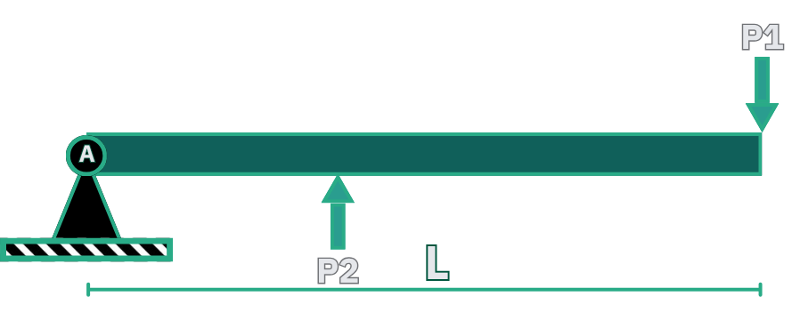
Application 1: Pantograph Arm of Electric Train (Electromechanical)
An electric train pantograph arm maintains contact with overhead power lines through a spring-loaded mechanism. Real pantographs use a pin joint at the base with spring forces to provide the upward contact pressure, allowing the arm to articulate and adapt to varying wire heights.
Set this beam and section in the simulator and read the maximum bending stress directly:
Hollow steel tube: Outer Diameter (OD) = 50 mm, wall thickness = 4 mm
Total arm length: L = 1200 mm from pin joint A to contact point P1
Spring location P2: 300 mm from pin joint A
Loading Conditions:
Wire contact force: P1 = 800 N downward at tip (reaction from overhead cable)
Spring force: F_spring (P2) = ? (to be determined from equilibrium)
Cross-Section Properties:
Second moment of area: I = 2.45 × 10⁶ mm⁴
Distance to extreme fiber: c = 25 mm
Section modulus: S = I/c = 98,000 mm³
Material & Safety:
Material: High-strength steel (σ_yield = 250 MPa)
Safety factor required: 3.0
Operating conditions: Dynamic contact with overhead wire at 600V DC
Step 1: Calculate Spring Force and Support Reactions
Click to reveal equilibrium calculations
Identify loading and support configuration:
Pin joint at A (x = 0): Provides vertical reaction R_A only (no moment resistance!)
Spring mechanism at x = 300 mm: Provides upward force F_spring
Wire contact at P₁ (x = 1200 mm): Downward reaction force = 800 N
Calculate required spring force using moment equilibrium about pin A:
(pin joint cannot resist moment)
Taking counterclockwise moments as positive:
✅
Physical meaning: Spring must provide 4× the contact force due to 4:1 lever arm ratio (1200/300)
Calculate pin reaction using vertical force equilibrium:
Negative sign means R_A acts downward (pin pulls down on the arm) ✅
Verify equilibrium:
Vertical forces: ✅
Moments about A: ✅
Key insight - comparison with fixed cantilever:
Fixed cantilever (incorrect model): Maximum moment (M = 960 N·m) at support A
Pin + Spring (correct model): No moment at A (pin cannot resist moment). Maximum moment will occur at the spring location where internal forces change!
Step 2: Shear Force Analysis
Click to reveal shear calculations at critical points
Region 1: Pin joint to spring (0 ≤ x < 0.3 m):
Applying force equilibrium on a section between pin and spring:
Negative indicates downward internal shear force
No applied loads in this region, so V remains constant ✅
Region 2: Spring to wire contact (0.3 m < x ≤ 1.2 m):
After passing the spring, the upward spring force adds to the reaction:
Positive indicates upward internal shear force
Remains constant until the wire contact point
At wire contact (x = 1.2 m), the 800 N downward force brings V back to zero ✅
Shear force jump at spring location (x = 0.3 m):
Just before spring:
Just after spring:
Jump magnitude: (equals spring force) ✅
Verify shear at wire contact:
At x = 1.2 m (after wire contact): ✅
Shear Force Diagram
Key observations:Two-region shear distribution: V = -2400 N from pin to spring, then V = +800 N from spring to wire
Discontinuity at spring: 3200 N upward jump where spring force is applied
Unlike fixed cantilever: Shear is NOT constant—changes sign at spring location
Step 3: Bending Moment Analysis
Click to reveal moment calculations at critical points
Method: Cut the beam at position x, sum moments of forces to the LEFT of the cut
At pin joint (x = 0):
Forces to the left: None (starting point)
Key insight: Pin joint cannot resist moment! ✅
Region 1 (0 < x < 0.3 m): Pin to spring
Forces to the left: R_A only
(in N·m when x in meters)
Linear increase in negative moment
At x = 0.3 m (spring location): ✅
Region 2 (0.3 m < x < 1.2 m): Spring to wire
Forces to the left: R_A and F_spring
(N·m)
At x = 0.3 m: (continuous at spring)
At x = 0.6 m (midspan):
At x = 0.9 m:
At x = 1.2 m (wire contact): ✅
Verify moment equilibrium:
At wire contact (x = 1.2 m), moment should equal zero (free end condition):
✅
Critical observation: Negative moments throughout indicate tension on top fiber and compression on bottom fiber. The beam curves downward (pantograph arm droops under wire contact force).
Bending Moment Diagram
Key observations:
Region 1 (0 to 0.3m): M(x) = -2400x (steep negative slope)
Region 2 (0.3m to 1.2m): M(x) = 800x - 960 (gentler positive slope)
Maximum moment magnitude: |M_max| = 720 N·m at spring location (x = 0.3 m)
Critical design location: Spring attachment point experiences highest bending stress
Step 4: Calculate Maximum Bending Stress
Click to reveal stress calculations
Apply flexural formula at critical section (spring location):
Alternative using section modulus:
✅
Stress distribution at spring attachment (x = 0.3 m):
Maximum tensile stress: +7.35 MPa (top fiber)
Maximum compressive stress: -7.35 MPa (bottom fiber)
Neutral axis stress: 0 MPa ✅
Step 5: Safety Factor Assessment
Click to reveal safety calculations
Calculate actual safety factor:
Compare with required safety factor:
Required SF = 3.0
Actual SF = 34.0 >> 3.0 ✅
Design adequacy assessment:
The pantograph arm is significantly over-designed with respect to static bending stress.
This high safety margin (>10× required) is intentional for several reasons:
Endurance limit for steel: ~125 MPa (50% of yield for high-cycle fatigue)
Maximum stress (7.35 MPa) is far below endurance limit
High safety factor (SF = 34) provides adequate fatigue life margin ✅
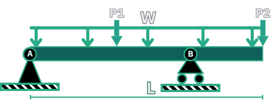
Application 2: Crane Jib with Overhang Loading (Mechanical)
An industrial crane jib beam supports a hoist mechanism with multiple load points typical in material handling systems. This analysis demonstrates complex loading scenarios with both positive and negative bending moments.
🔧 Equivalent System Model
Given:
Steel I-beam: 150 mm × 100 mm × 8 mm (I = 8.2 × 10⁶ mm⁴, c = 75 mm)
Span: 3000 mm between supports A and B
Overhang: 1000 mm beyond support B
Load 1: P₁ = 5000 N at 1500 mm from A (midspan)
Load 2: P₂ = 3000 N at end of overhang
Load 3: Distributed load W = 800 N/m over entire length (beam self-weight + attachments)
Design is conservative with SF = 5.94, well above required SF = 2.5
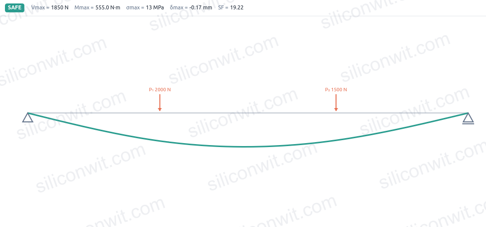
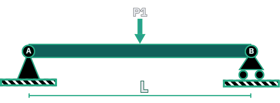
Application 3: 3D Printer Gantry Rail (Mechatronics)
A 3D printer gantry rail supports a moving print head assembly that traverses the build platform. The rail experiences a concentrated load as the print head moves to different positions during printing. We need to determine which position creates the worst-case bending stress.
🔧 Equivalent System Model
Geometric Configuration:
Aluminum extrusion beam: Span L = 1200 mm between supports
Support A at x = 0 mm (left end)
Support B at x = 1200 mm (right end)
Loading Positions to Analyze:
Print head weight: P = 250 N (includes extruder, hotend, cooling fans)
Position 1: Left quarter-point (x = 300 mm from support A)
Position 2: Midspan (x = 600 mm from support A)
Position 3: Right quarter-point (x = 900 mm from support A)
Conclusion: The large cross-section is needed for stiffness (deflection control), not strength. Bending stress is very low compared to material strength.
Summary and Next Steps
In this lesson, you learned to:
Apply the flexural formula σ = My/I for bending stress calculation
Identify neutral axis location and stress distribution patterns
Calculate section properties for common cross-sections
Design beams to meet both strength and safety factor requirements
Key Design Insights:
Maximum stress occurs at extreme fibers
Section modulus S = I/c determines bending capacity
Tall sections are much more efficient in bending
Critical Formula:
Coming Next: In Lesson 2.3, we’ll analyze beam deflections and stiffness, exploring how to calculate elastic deformations in CNC spindles under cutting loads for precision control applications.


Comments