Master beam deflection analysis through real-world precision applications: PCB sagging under component weight, mobile C-arm fluoroscopy positioning accuracy, and CNC gantry rail stiffness. Learn elastic curve equations, support configuration effects (fixed-fixed, cantilever, simply supported), and stiffness design strategies for electronics, medical, and manufacturing systems.
Learning Objectives
By the end of this lesson, you will be able to:
Calculate beam deflections using standard formulas for various loading and support conditions
Apply superposition principles for complex loading scenarios
Analyze how support configurations (cantilever, simply supported, fixed-fixed) affect deflection behavior
Design structural members to meet stiffness requirements for precision applications
Engineering Challenge: Deflection in Precision Systems
Beam deflection is a critical design consideration across diverse engineering applications—from electronic circuit boards sagging under component weight, to medical imaging C-arms requiring sub-millimeter positioning accuracy, to CNC machine gantry rails maintaining cutting precision. Understanding deflection theory enables engineers to predict elastic deformations, establish appropriate design limits, and optimize structural stiffness for functionality and reliability.
The Universal Deflection Challenge
Across mechanical, electronics, and medical engineering, beam structures must resist deflection to maintain:
Engineering Question: How do we predict beam deflections under various loading conditions, assess them against application-specific limits, and design cost-effective solutions that meet stiffness requirements?
Why Deflection Analysis Matters
Consequences of Inadequate Stiffness Design:
Electronics: Solder joint cracking from excessive PCB flexure under component weight
Medical imaging: Blurred images and artifacts from C-arm deflection during surgical procedures
Precision machining: Positioning errors in CNC systems compromising part tolerances and surface finish
Material waste: Over-design from conservative assumptions without analytical validation
Benefits of Proper Deflection Analysis:
Predictable performance within established tolerance bands
Optimized material usage through accurate stiffness calculations
Informed design trade-offs between weight, cost, and performance
Application-specific deflection limits tailored to functional requirements (not arbitrary rules)
Fundamental Theory: Elastic Beam Deflections
The Elastic Curve Equation
When a beam bends under load, it forms a curved shape called the elastic curve. Understanding this curve is the key to predicting deflections.
📋 Deriving the Elastic Curve Equation
Step 1: Relationship between curvature and moment
From solid mechanics, a bending moment M causes a beam to curve. The fundamental relationship is:
Where:
= Radius of curvature (m) - the radius of the circle that the bent beam follows at any point
= Bending moment as a function of position along the beam (N·m)
= Young’s modulus - material stiffness (Pa)
= Second moment of area - geometric property of cross-section (m⁴)
= Flexural rigidity - combined stiffness of the beam (N·m²)
What this means: A larger bending moment creates tighter curvature (smaller radius ). A stiffer beam (higher ) resists curvature more (larger radius ).
Step 2: Converting curvature to deflection
From calculus, the curvature of a curve is:
This exact formula is complex, but for small deflections (which applies to most engineering beams), the slope is very small, so .
Small deflection approximation: When slopes are small (typically less than 10°), we can simplify:
Step 3: Combining the relationships
Setting the two expressions for curvature equal:
This is the fundamental elastic curve equation!
Physical Meaning:
Left side = curvature of the deflected beam (how much it bends)
Right side = bending moment divided by flexural rigidity
Key insights:
Where moment is large → curvature is large → beam bends more sharply
Where moment is zero → curvature is zero → beam is straight
Higher → less curvature for same moment → stiffer beam
This equation tells us: “The shape the beam takes is determined by the moment distribution along its length”
Double Integration Method
The double integration method is a systematic procedure to find beam deflections by integrating the elastic curve equation twice.
Determine the bending moment as a function of position along the beam using equilibrium equations (from earlier lessons).
Example: For a cantilever beam with tip load P:
Step 2: Write the elastic curve equation
For our cantilever example:
Step 3: First integration → Slope equation
Integrate both sides with respect to x:
This gives:
📈 Slope Equation
Physical Meaning:
is the slope (angle) of the deflected beam at position x
is an integration constant determined by boundary conditions
The slope tells us how tilted the beam is at each point
For our cantilever example:
Step 4: Second integration → Deflection equation
Integrate the slope equation to get deflection:
This gives:
📉 Deflection Equation
Physical Meaning:
is the deflection (vertical displacement) of the beam at position x
represents the contribution from the initial slope
is another integration constant (initial deflection)
The deflection tells us how far the beam has moved from its original position
For our cantilever example:
Step 5: Apply boundary conditions to find C₁ and C₂
Use the known conditions at supports to solve for the integration constants (see Boundary Conditions tab).
For our cantilever (fixed at x=0):
At x = 0: y = 0 (no deflection at fixed end)
At x = 0: dy/dx = 0 (no rotation at fixed end)
From dy/dx = 0 at x = 0:
From y = 0 at x = 0:
Final deflection equation:
Tip deflection (at x = L):
The negative sign indicates downward deflection (same direction as load P).
Boundary conditions are the known constraints at supports that allow us to solve for the integration constants C₁ and C₂.
🔗 Simply Supported (Pin-Roller)
Physical constraints:
Pin and roller supports prevent vertical movement but allow rotation
No external moments are applied at the supports
Mathematical boundary conditions:
At both supports (x = 0 and x = L): (zero deflection)
At both supports: which means (zero moment)
What this means:
The beam can’t move up or down at support points
The beam is free to rotate at supports (dy/dx ≠ 0)
The beam touches but doesn’t “stick” to the supports
Example application:
For a simply supported beam, use y(0) = 0 and y(L) = 0 to find C₁ and C₂.
🔒 Cantilever (Fixed-Free)
Physical constraints:
Fixed end prevents both movement and rotation (fully restrained)
Free end has no constraints
Mathematical boundary conditions:
At fixed end (x = 0): (zero deflection)
At fixed end (x = 0): (zero slope/rotation)
Alternative conditions at free end (if needed):
At free end (x = L): means (unless there’s an applied moment)
At free end (x = L): equals applied load
What this means:
The beam is completely locked at the fixed end - can’t move or rotate
The free end can deflect and rotate freely
Maximum deflection occurs at the free end
Example application:
Use y(0) = 0 and dy/dx(0) = 0 to find C₁ and C₂ (as shown in Integration Steps).
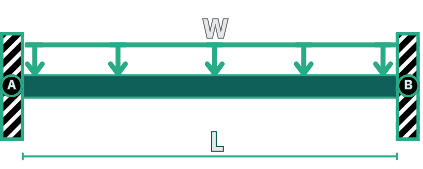
🔗🔒 Fixed-Fixed (Clamped-Clamped)
Physical constraints:
Both ends are rigidly clamped (like built-in beams)
Neither end can move or rotate
Mathematical boundary conditions:
At both ends (x = 0 and x = L): (zero deflection)
At both ends (x = 0 and x = L): (zero slope/rotation)
What this means:
The beam is fully locked at both ends
This creates reaction moments at the supports (not just forces)
The beam is much stiffer than simply supported (up to 5× stiffer)
Maximum deflection occurs near the center
Example application:
Use y(0) = 0, dy/dx(0) = 0, y(L) = 0, and dy/dx(L) = 0. Note: For complex loading, you may need to find reaction moments first using equilibrium.
Summary table:
Support Type
Deflection y
Slope dy/dx
Moment M
Pin/Roller
= 0 (fixed)
≠ 0 (free)
= 0 (free to rotate)
Fixed/Clamped
= 0 (fixed)
= 0 (fixed)
≠ 0 (reaction moment)
Free end
≠ 0 (free)
≠ 0 (free)
= 0 (no applied moment)
These formulas are the results of applying the double integration method to common beam configurations. You can use them directly without re-deriving each time.
🎢 Standard Deflection Formulas
Cantilever Beams (Fixed-Free):
Point load P at tip: (at free end, x = L)
Derivation basis: Fixed at x=0 (y=0, dy/dx=0), moment M(x) = -P(L-x)
Uniform load w: (at free end, x = L)
Derivation basis: Fixed at x=0, moment M(x) = -w(L-x)²/2
Simply Supported Beams (Pin-Roller):
Center point load P: (at center, x = L/2)
Derivation basis: Supports at x=0 and x=L (y=0 at both), symmetric moment distribution
Note: 16× stiffer than cantilever with same load!
Uniform load w: (at center, x = L/2)
Derivation basis: Supports at x=0 and x=L, parabolic moment distribution
Fixed-Fixed Beams (Clamped-Clamped):
Center point load P: (at center, x = L/2)
Derivation basis: Both ends clamped (y=0, dy/dx=0), develops reaction moments
Note: 4× stiffer than simply supported, 64× stiffer than cantilever!
Uniform load w: (at center, x = L/2)
Derivation basis: Both ends clamped, reaction moments reduce midspan moment
Understanding the denominators:
Notice the patterns in denominators:
Cantilever point load: 3 (least stiff - only one constraint)
Simply supported: at center for symmetric loading (x = L/2)
Fixed-fixed: at or near center for symmetric loading (x = L/2)
When to use each formula:
Use these directly when your loading matches exactly
For other cases, use superposition (next section) or double integration method
Always verify: units must work out to length (meters)
Superposition Principle
When a beam experiences multiple loads simultaneously, we can find the total deflection by calculating each load’s contribution separately and then adding them together.
📊 Superposition for Beam Deflections
The principle:
Why this works:
The elastic curve equation is linear in deflection y
This means: deflection from load A + deflection from load B = deflection from both loads together
This is only valid for small deflections and elastic behavior (no yielding)
Step-by-step procedure:
Identify each load separately (point loads, distributed loads, moments)
Calculate deflection from each load using standard formulas (treating other loads as zero)
Add all deflections algebraically (pay attention to signs: downward = negative, upward = positive)
The result is the total deflection at any point of interest
Example: Simply supported beam with center point load P AND uniform load w
For a beam with length L, both loads act together:
Deflection from point load P alone:
Deflection from uniform load w alone:
Total deflection at center:
Important notes:
All deflections must be calculated at the same point (e.g., midspan, or a specific location x)
Use the same coordinate system for all loads
If loads act in opposite directions, their deflections have opposite signs
This method works for any linear-elastic beam problem
When superposition is especially useful:
Complex loading patterns (multiple point loads + distributed loads)
Unsymmetric loading (loads at different positions)
Combination of loads and applied moments
Finding deflection at specific points (not just maximum)
Limitations:
Only valid for linear elastic materials (stress ∝ strain)
Only valid for small deflections (slope 1)
Cannot use if beam yields or deforms plastically
Cannot use if deflections are large enough to change geometry significantly
Application 1: PCB Sagging in Rack (Electronics)
A printed circuit board (PCB) is mounted between two supports in an electronics rack. The PCB experiences deflection due to the combined weight of mounted components distributed across its surface.
Set this beam in the simulator and read the maximum deflection as you vary the span:
Fixed-fixed is 5× stiffer (ratio: 5/384 ÷ 1/384 = 5). Although fixed-fixed beams are statically indeterminate (cannot solve for reaction moments using equilibrium alone), this formula is pre-derived using the 4 boundary conditions (y=0 and dy/dx=0 at both ends). In practice: Use this formula directly. You don’t need to solve the indeterminate system yourself.
Convert units to SI:
L = 200 mm = 0.2 m
w = 60 N/m (distributed load intensity - already calculated from 12 N total / 0.2 m span)
E = 20 GPa = 20 × 10⁹ Pa
I = 3.413 × 10⁻¹¹ m⁴ ✅
Note: The formula requires distributed load intensity w (N/m), not total load W (N).
Calculate maximum deflection at midspan:
✅
Calculate deflection as percentage of span:
✅
Step 2: Relate Deflection to Solder Joint Reliability
Click to reveal solder joint analysis
Understand PCB deflection limits:
Industry standards for PCB deflection:
IPC-2221 guideline: Maximum deflection less than L/100 for boards with components
Conservative limit: L/150 for boards with sensitive components (BGAs, fine-pitch ICs)
Calculated deflection: L/546 ✅
Assess deflection against standards:
Current deflection: 0.366 mm = L/546
Recommended limit: L/100 = 2.0 mm
Conservative limit: L/150 = 1.33 mm
Status: Excellent - well within both limits ✅
The PCB deflection is excellent, with large safety margins:
vs L/100 limit: 0.366 mm vs 2.0 mm (82% margin) ✅
vs L/150 limit: 0.366 mm vs 1.33 mm (72% margin) ✅
Solder joint stress mechanisms:
How deflection damages solder joints:
Bending-induced strain: PCB curvature creates tensile strain on component leads and solder
Cyclic loading: Temperature cycling + mechanical deflection = fatigue
Crack initiation: Repeated stress causes solder microcracks at component interfaces
Design principle: Place heaviest components near supports
Move heavy components (transformers, heatsinks, connectors) to board edges near supports
Concentrate lightweight components (resistors, capacitors) near center
This reduces effective load at maximum deflection point
Estimated improvement: 20-30% deflection reduction (depends on component distribution)
Trade-offs:
✅ No material or structural changes needed
✅ Zero cost solution
❌ Limited by circuit routing constraints
❌ May conflict with thermal management
Assessment and recommendations:
Current design status:
Deflection: 0.366 mm = L/546
The current fixed-fixed mounting already provides excellent stiffness ✅
Meets IPC-2221 standard (L/100) with 82% margin
Meets conservative limit (L/150) with 72% margin
If additional improvements are needed (high-reliability applications):
Keep current design - it’s already excellent for most applications
If ultra-high reliability required (L/200 or better):
Increase to 2.0 mm thickness → δ = 0.187 mm (L/1070)
Or add edge stiffeners → δ = 0.215 mm (L/930)
Optimize component placement - always a good practice regardless
Key insight: Fixed-fixed mounting is 5× stiffer than simply supported would be, making this design inherently robust.
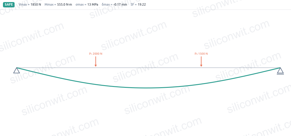
Application 2: Mobile C-Arm Fluoroscopy System (Mechatronics/Medical)
A mobile C-arm fluoroscopy system is used in operating rooms and clinics for real-time X-ray imaging during surgical procedures. The C-shaped cantilever arm extends from a vertical support column, holding the X-ray source on one end and the detector panel on the opposite end. The arm must maintain precise alignment between source and detector despite their combined weight to produce clear images.
🔧 Equivalent System Model
Given:
Cantilever arm length (from column to detector): L = 1.2 m
Tip load: P = 800 N (combined X-ray source ~400 N + detector assembly ~400 N at effective center)
Cross-section: Hollow steel C-shaped channel
Outer diameter (circular arc approximation): OD = 120 mm
Wall thickness: t = 8 mm
Inner diameter: ID = OD - 2t = 104 mm
Material: High-strength steel (E = 210 GPa)
Step 1: Calculate Tip Deflection
Click to reveal tip deflection calculations
Identify the deflection formula for cantilever beam with tip load:
For concentrated load P at the free end of a cantilever:
Where:
P = tip load (N)
L = cantilever length (m)
E = Young’s modulus (Pa)
I = second moment of area (m⁴)
Calculate second moment of area for hollow circular section:
✅
Convert units to SI:
P = 800 N
L = 1.2 m
E = 210 GPa = 210 × 10⁹ Pa
I = 4.44 × 10⁻⁶ m⁴ ✅
Calculate tip deflection:
✅
Calculate deflection as fraction of span:
✅
Step 2: Comment on Stiffness Requirements for Imaging Precision
Click to reveal imaging precision analysis
C-arm fluoroscopy precision requirements:
Mobile C-arm fluoroscopy systems require:
Spatial resolution: 1.0-2.0 mm (ability to visualize bones, instruments, contrast agents)
Source-detector alignment: ±1.0 mm (to maintain image geometry and prevent distortion)
Image intensifier positioning: ±0.5-1.0 mm (for consistent image quality)
Detector pixel size: 0.2-0.4 mm (typical flat-panel detector element spacing)
Note: C-arms have less stringent requirements than CT scanners because they produce 2D projection images rather than 3D reconstructions ✅
Why the C-shape design?
Structural efficiency: The curved C-section provides a continuous load path from source to detector, distributing loads more evenly than a straight cantilever
Simplification for analysis: We model the C-arm as an equivalent straight cantilever beam because the bending behavior is dominated by the cantilever length (base to detector), and the curved geometry has similar flexural rigidity to a straight beam of the same cross-section. This simplification is valid for calculating maximum deflection at the detector end ✅
Impact of arm deflection on image quality:
Calculated deflection: 0.494 mm
Effects on imaging:
Source-detector misalignment: 0.494 mm deflection creates minor geometric distortion
Focal point stability: Acceptable for real-time fluoroscopy guidance
Image sharpness: Within tolerance for surgical navigation and fracture reduction
Overall assessment: Borderline acceptable, but close to design limits ⚠️
Deflection contribution to total positioning error:
Total positioning error budget:
Mechanical deflection (static): 0.494 mm (calculated) ✅
C-arm rotation clearances: ±0.3 mm (bearing play and orbital track tolerance)
Thermal expansion: ±0.2 mm (during extended procedures)
Vibration amplitude: ±0.15 mm (from positioning motors and floor vibration)
Total error (RSS): √(0.494² + 0.3² + 0.2² + 0.15²) = 0.63 mm ⚠️
Assessment against precision requirements:
Current design performance:
Required source-detector alignment: ±1.0 mm
Calculated total error: 0.63 mm
Safety margin: 37% margin below requirement ✅
However, consider dynamic loading:
During repositioning: Dynamic loads can increase deflection by 1.5-2×
Estimated maximum deflection: 0.494 × 1.5 = 0.74 mm
Total error with dynamics: ~0.86 mm (14% margin remaining) ⚠️
Impact on imaging:
✅ Acceptable for: Orthopedic procedures, vascular imaging, general fluoroscopy
⚠️ Marginal for: Neuro-interventional procedures requiring high precision
❌ Insufficient for: Cardiac catheterization labs (require less than 0.3 mm deflection)
Stiffness-driven design considerations:
Why stiffness dominates C-arm design:
Stress is not the issue: Calculated bending stress ≈ 12 MPa ≪ yield of 350+ MPa
Deflection controls design: Must maintain source-detector alignment within 1 mm
Dynamic effects: C-arm repositioning creates transient loads and vibrations
Design is stiffness-limited, not strength-limited ✅
Current design meets basic requirements but has limited safety margin ⚠️
Recommendations for improved precision:
To achieve high-precision target (0.25 mm deflection for cardiac/neuro applications):
Keep OD = 120 mm, increase wall to t = 12 mm (ID = 96 mm)
I = π(120⁴-96⁴)/64 = 6.01×10⁶ mm⁴
Improvement: δ reduces to 0.37 mm ✅
Trade-off: 50% heavier, reduced internal cable routing space, still marginal for high-precision
Option 3: Add counterweight system
Reduce net tip load from 800 N to ~296 N (63% counterweighting)
Improvement: δ reduces to 0.18 mm ✅
Trade-off: Increases system weight, requires larger motor torques
Option 4: Use carbon fiber composite
Carbon fiber/epoxy: E = 140 GPa (67% of steel), ρ = 1600 kg/m³ (20% of steel)
With OD = 140 mm, t = 10 mm: I = 8.68×10⁶ mm⁴, lighter weight
Improvement: δ reduces to 0.38 mm, 50% weight reduction ✅
Trade-off: Higher cost, X-ray transparency concerns (good for imaging, bad for structural visibility), still marginal
Recommended solution: For general fluoroscopy, current design is adequate. For high-precision cardiac/neuro applications, either increase diameter to 149 mm or add 63% counterweighting to achieve less than 0.25 mm deflection target.
Step 3: Establish Allowable Deflection Limits for Medical Imaging
Click to reveal allowable deflection analysis
Understand the L/250 deflection limit rule:
Common engineering deflection limits:
L/360: Very stiff structures (plastered ceilings, brittle finishes)
L/250: General structural members (beams, floor joists)
L/180: Flexible structures (roof beams with flexible finishes)
The L/250 rule is a general guideline for structures where visible sagging or functional issues should be avoided ✅
Apply L/250 rule to C-arm:
✅
Compare calculated deflection to L/250 limit:
Calculated deflection: 0.494 mm
L/250 limit: 4.8 mm
Ratio: 0.494 / 4.8 = 0.103 (10.3% of allowable)
Deflection EASILY PASSES the general L/250 structural rule ✅
Critical assessment: Is L/250 appropriate for C-arm fluoroscopy?
NO - L/250 is far too lenient for precision medical imaging. However, it’s useful as a baseline structural check.
Why L/250 is inadequate for medical imaging:
L/250 is designed for structural deflection limits (preventing damage, visible sagging)
L/250 = 4.8 mm would cause unacceptable image distortion and blur
For C-arms, application-specific limits of 0.5-1.0 mm are more appropriate ✅
Establish appropriate deflection limit for C-arm fluoroscopy:
Recommended deflection limit hierarchy for C-arms:
High-precision interventional (cardiac/neuro):
Target: L/4000 to L/6000 = 0.20-0.30 mm
Maximum: L/2400 = 0.50 mm
Current design: 0.494 mm → fails maximum limit ❌
Standard surgical fluoroscopy:
Target: L/2000 = 0.60 mm
Maximum: L/1200 = 1.0 mm
Current design: 0.494 mm → acceptable (51% margin) ✅
General orthopedic/trauma imaging:
Target: L/1200 = 1.0 mm
Maximum: L/800 = 1.5 mm
Current design: 0.494 mm → excellent (67% margin) ✅
Design adequacy summary:
Application Type
Target Limit
Maximum Limit
Calculated
Status
L/250 structural rule
—
4.8 mm
0.494 mm
✅ Pass (90% margin)
High-precision interventional
0.25 mm
0.50 mm
0.494 mm
❌ Fail (exceeds by 1%)
Standard surgical
0.60 mm
1.0 mm
0.494 mm
✅ Good (51% margin)
General orthopedic
1.0 mm
1.5 mm
0.494 mm
✅ Excellent (67% margin)
Conclusion: The L/250 structural rule is not appropriate as a design criterion for medical imaging equipment, but it serves as a useful baseline check. The current design is adequate for general surgical and orthopedic fluoroscopy but fails requirements for high-precision cardiac/neuro interventional procedures.
Application-specific design recommendations:
For general surgical applications (current design is adequate):
Current δ = 0.494 mm meets requirements ✅
Consider 20-30% safety margin for dynamic loads
Monitor deflection during service life (bearing wear increases deflection)
For high-precision interventional applications (improvement needed):
Target δ less than 0.25 mm (requires ~50% deflection reduction)
Option 1: Increase OD to 149 mm (t=8mm) → δ = 0.25 mm ✅
Option 2: Increase wall thickness to 12 mm → δ = 0.37 mm (still insufficient) ❌
Key insight: Unlike general structural design where L/250 is a universal rule, medical imaging requires application-specific deflection limits based on image quality requirements. C-arms for orthopedic surgery can tolerate 1.0 mm deflection, while cardiac catheterization labs require less than 0.3 mm - a 3× difference driven by clinical needs, not arbitrary rules.
A CNC router or laser cutter uses a simply supported beam as the Y-axis gantry support rail. The moving gantry (carrying motors, linear guides, and tool head) creates a concentrated load that travels along the beam during machining operations. The rail must maintain stiffness to preserve cutting accuracy.
🔧 Equivalent System Model
Given:
Rail length (Y-axis span): L = 1.0 m
Point load at center: P = 500 N (gantry assembly: motors + linear guides + tool head)
Cross-section: Rectangular steel rail/extrusion
Width: b = 80 mm
Height: h = 30 mm
Area: A = 2400 mm²
Material: Steel (E = 210 GPa)
Step 1: Calculate Maximum Midspan Deflection
Click to reveal maximum deflection calculations
Identify the deflection formula for simply supported beam with center point load:
For concentrated load P at the center of a simply supported span:
Where:
P = point load at center (N)
L = span length (m)
E = Young’s modulus (Pa)
I = second moment of area (m⁴)
Note: This formula gives maximum deflection at midspan (x = L/2) where the load is applied ✅
Calculate second moment of area for rectangular section:
✅
Convert units to SI:
P = 500 N
L = 1.0 m
E = 210 GPa = 210 × 10⁹ Pa
I = 1.80 × 10⁻⁷ m⁴ ✅
Calculate maximum deflection at midspan:
✅
Calculate deflection as fraction of span:
✅
This represents good stiffness for CNC applications (L/3623 is better than typical L/1000 minimum)
Step 2: Compare with Other Support Configurations
Click to reveal support configuration comparison analysis
Calculate deflection for fixed-fixed configuration with same loading:
Fixed-fixed configuration: Both ends clamped (no rotation or translation)
Deflection formula for fixed-fixed beam with center point load:
Calculation:
✅
Calculate deflection for cantilever configuration with same loading:
Cantilever configuration: One end fixed, load at free end (tip)
Deflection formula for cantilever with tip point load:
Calculation:
✅
Comparative analysis of support configurations:
Configuration
Deflection Formula
Calculated Deflection
Relative Stiffness
Fixed-Fixed
PL³/(192EI)
0.069 mm
4.0× stiffer than simply supported ✅
Simply Supported
PL³/(48EI)
0.276 mm (baseline)
1.0× ✅
Cantilever
PL³/(3EI)
4.41 mm
0.063× (16× more flexible)
Understand the physics of support stiffness:
Fixed-Fixed beam:
✅ No rotation at supports (moment resistance at both ends)
✅ No translation at supports (full constraint)
✅ Develops reaction moments at supports (counteracts midspan sagging)
✅ Midspan moment reduced significantly by support moments
Result: 4× stiffer than simply supported ✅
Simply supported beam (current design):
✅ No translation at supports
❌ Free rotation at supports (no moment resistance)
✅ Allows thermal expansion (roller end can slide longitudinally)
✅ Easier to manufacture and assemble
Result: Baseline stiffness - good balance of performance and practicality ✅
Cantilever beam:
✅ No rotation or translation at fixed end
❌ Free end completely unconstrained
❌ Maximum moment at fixed end, zero at tip
Result: 16× more flexible than simply supported ✅
Deflection comparison factors:
Simply supported vs. Fixed-fixed:
Stiffness ratio: 1:4 (fixed-fixed is 4× stiffer)
Formula relationship: vs.
Coefficient ratio: 192:48 = 4:1 ✅
Simply supported vs. Cantilever:
Stiffness ratio: 16:1 (simply supported is 16× stiffer)
Formula relationship: vs.
Coefficient ratio: 48:3 = 16:1 ✅
Practical implications for CNC gantry design:
Why simply supported is commonly used:
Thermal management: Roller end allows linear thermal expansion without inducing stress
Ease of assembly: Simpler mounting than fixed-fixed (no moment connections required)
Cost-effective: Standard linear rail mounting blocks provide pin-roller support
Good stiffness: 16× better than cantilever, adequate for most CNC applications ✅
When to use other configurations:
Fixed-fixed: When maximum stiffness is required (high-precision machining, heavy cutting forces)
Requires rigid moment connections at both ends
Must account for thermal expansion stresses
Cantilever: When only one-side mounting is possible (space constraints, overhung load)
16× more flexible - avoid unless necessary
Simply supported: Standard choice for most CNC machines (good balance) ✅
Step 3: Discuss Stiffness Improvement Strategies
Click to reveal stiffness enhancement strategies
Strategy 1: Increase rail height (most effective for cost)
Deflection is proportional to I = bh³/12, so height has cubic effect:
Option: Increase height from 30 mm to 40 mm
✅
Improvement: 58% deflection reduction (from 0.276 mm to 0.116 mm)
Trade-offs:
✅ Most cost-effective improvement per added material


Comments