Lesson 1: Kinematic Joints and Degrees of Freedom in 3D Systems

Contributors

Become Contributor

Learn kinematic joint analysis through modular robot design, covering all joint types, degrees of freedom calculations, and constraint relationships in 3D mechanical systems.

🎯 Learning Objectives

By the end of this lesson, you will be able to:

1. Classify all kinematic joint types and their motion characteristics in 3D space
2. Calculate degrees of freedom for spatial mechanisms using Grübler's equation
3. Analyze constraint relationships and mobility in modular robotic systems
4. Design joint libraries for reconfigurable mechatronic applications

🔧 Real-World System Problem: Modular Robot Joint Library

System Description

Universal Modular Robot System Components:

• Standardized Joint Library (revolute, prismatic, spherical, universal joints)
• Modular Link Segments (variable lengths and cross-sections)
• Quick-Connect Interfaces (mechanical and electrical coupling)
• Central Control System (coordinates multiple joint types)
• Reconfiguration Tools (rapid system redesign capabilities)

The Joint Analysis Challenge

When designing modular systems, engineers face critical decisions:

Engineering Question: How do we systematically analyze and catalog the motion capabilities of different joint types to create a comprehensive modular robot library?

📚 Fundamental Theory: Joint Types and Constraints

Classification of Kinematic Joints

In 3D space, kinematic joints can be classified by the number of constraints they impose:

• Lower DoF Pairs
• Higher DoF Pairs
• Special Joints
• Extreme Cases

Lower pairs maintain surface contact between links:

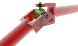
🔄 Revolute (Hinge) Joint

Motion: 1 rotational DoF about fixed axis
Constraints: 5 (removes 2 translations + 1 rotation perpendicular to axis + 2 rotations about other axes)
DoF: 1

Motion	X-Axis	Y-Axis	Z-Axis
Translation	❌	❌	❌
Rotation	❌	✅	❌

Applications: Robot arm joints, wheel axles, door hinges

↕️ Prismatic Joint

Motion: 1 translational DoF along fixed axis
Constraints: 5 (removes 2 translations perpendicular to axis + 3 rotations)
DoF: 1

Motion	X-Axis	Y-Axis	Z-Axis
Translation	❌	❌	✅
Rotation	❌	❌	❌

Applications: Linear actuators, telescoping mechanisms, sliding doors

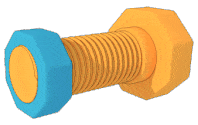
🌀 Helical Joint

Motion: Combined rotation and translation (screw motion)
Constraints: 5 (coupled rotation-translation motion)
DoF: 1

Motion	X-Axis	Y-Axis	Z-Axis
Translation	❌	❌	✅
Rotation	❌	❌	✅

Applications: Lead screws, propeller shafts, screw jacks

Degrees of Freedom Analysis

Systematic Joint Analysis Process

1. Identify all links in the mechanism (include ground as link 1)

2. Classify each joint type and determine constraints imposed

3. Apply Grübler’s equation to calculate total degrees of freedom

4. Verify mobility through physical reasoning and constraint analysis

5. Check for special cases (redundant constraints, passive joints)

🔧 Application: Modular Robot Joint Library Design

Let’s analyze various joint combinations for a reconfigurable robot system.

System Parameters:

• Universal modular robot platform with interchangeable joints
• Standard link lengths: L = 200 mm, 400 mm, 600 mm
• Joint library includes: revolute (R), prismatic (P), spherical (S), universal (U), cylindrical (C)
• Maximum system complexity: n ≤ 8 links
• Target applications: assembly, welding, material handling
• Safety requirement: No uncontrolled motion modes

Configuration 1: Serial Chain Analysis

Configuration 2: Complex Joint Analysis

Configuration 3: Parallel Mechanism Analysis

📊 Joint Library Analysis Summary

🎯 Advanced Analysis: Constraint Relationships

Series vs. Parallel Constraints

R + R + R = 1 + 1 + 1 = 3 DoF
R + P + R = 1 + 1 + 1 = 3 DoF
S + R + R = 3 + 1 + 1 = 5 DoF

Special Considerations

🛠️ Design Guidelines for Joint Selection

Selection Criteria Matrix

📋 Summary and Next Steps

In this lesson, you learned to:

1. Classify kinematic joints by their constraint characteristics and DoF
2. Calculate mechanism mobility using Grübler’s equation systematically
3. Analyze series, parallel, and hybrid joint configurations
4. Design modular joint libraries for specific applications

Key Design Insights:

• Each joint type provides specific motion capabilities
• DoF analysis predicts mechanism mobility
• Series joints add DoF, parallel joints add constraints

Critical Formula: (Grübler’s equation for spatial mechanisms)

Coming Next: In Lesson 2, we’ll develop the mathematical foundations for spatial motion by studying planar transformations using complex analysis and homogeneous coordinates through SCARA robot programming.