Master shear force and bending moment analysis through real-world industrial beam structures: robotic arm cantilevers, conveyor support systems, and solar tracker mechanisms. Learn load distribution analysis, diagram construction techniques, and critical section identification essential for safe structural design across mechatronics and automation systems.
Learning Objectives
By the end of this lesson, you will be able to:
Construct shear force and bending moment diagrams for cantilever, simply supported, and overhanging beam configurations
Identify critical sections with maximum shear and moment values across diverse loading conditions
Apply equilibrium principles to analyze beams under point loads, distributed loads, and combined loading scenarios
Determine reaction forces for different support types including fixed, pinned, and roller supports
Real-World Engineering Challenge: Beam Analysis in Industrial Automation Systems
Industrial automation systems rely on structural beam elements that must safely support complex loading conditions. Understanding how internal forces and moments distribute along beam structures is fundamental to preventing failure, optimizing material usage, and ensuring reliable performance across mechatronics, material handling, and renewable energy applications.
Industrial Beam Applications
Common Beam Structures in Automation:
Robotic Arms (cantilever beams supporting payloads and end-effectors)
Conveyor Support Beams (simply supported beams carrying multiple concentrated loads)
Solar Tracker Arms (overhanging beams managing distributed loads plus equipment forces)
The Structural Challenge
All industrial beam structures experience internal shear forces and bending moments that determine structural adequacy. Different support types (fixed, pinned, roller) and loading patterns (point loads, distributed loads, combined) create varying internal force distributions requiring careful analysis for safe design.
Engineering Question 1: How do we determine where maximum bending stresses occur in different beam configurations and what governs the critical design section?
Engineering Question 2: How do support types and loading patterns affect internal force distributions and structural requirements?
Engineering Question 3: What analytical tools enable optimized designs that balance safety, cost, and performance?
Why Beam Analysis Matters
Consequences of Inadequate Analysis:
Structural failure causing downtime, equipment damage, and safety hazards
Over-designed structures wasting material and increasing costs
Benefits of Proper Analysis:
Safe, reliable structures with appropriate safety factors
Material optimization through accurate critical section identification
Foundation for advanced analysis including stress and deflection prediction
Fundamental Theory: Shear Force and Bending Moment
Basic Beam Concepts
Before analyzing shear forces and bending moments, it’s essential to understand how beams are supported. The type of support determines which movements and rotations are allowed or prevented, directly affecting the reaction forces and internal stresses.
Common Support Types:
Pinned Support (Hinge)
✅ Allows rotation at the connection
❌ Prevents translation (both horizontal and vertical movement)
Reactions: Provides both vertical and horizontal reaction forces (2 unknowns: Rx, Ry)
Common applications: Used in joints of robotic arms, mechanical linkages, and hinged enclosures where controlled rotation is needed
Roller Support
✅ Allows rotation at the connection
✅ Allows translation in one direction (typically horizontal)
Reactions: Provides only vertical reaction force (1 unknown: Ry)
Common applications: Found in systems like conveyor supports, linear guides, and structures accommodating thermal or mechanical expansion
Fixed Support (Built-in/Clamped)
❌ Prevents rotation at the connection
❌ Prevents translation (both horizontal and vertical movement)
Reactions: Provides vertical force, horizontal force, and moment (3 unknowns: Rx, Ry, M)
Common applications: Used in cantilevered robotic arms, rigidly mounted machine bases, and firmly fixed electronic equipment supports
When a beam is loaded transversely, internal forces develop to maintain equilibrium:
Shear Force (V): Internal force that resists sliding Bending Moment (M): Internal moment that resists rotation Normal Force (N): Internal axial force (usually zero in pure bending)
The fundamental relationship between load, shear, and moment:
📏 Beam Differential Equations
Where:
= distributed load intensity (N/m)
= shear force at position x (N)
= bending moment at position x (N·m)
Physical Meaning: These equations show how load affects shear force rate of change, and how shear force affects bending moment rate of change.
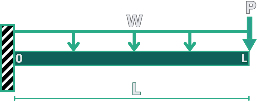
🛡️ Cantilever Beam (Fixed-Free)
For cantilever with distributed load w and point load P at tip:
Shear Force:
Bending Moment:
Key Characteristics:
Maximum shear and moment at fixed support
Zero shear and moment at free end
Linear shear variation, parabolic moment variation
⚖️ Simply Supported Beam (Pin-Roller)
For simply supported beam with central point load P:
Shear Force:
Bending Moment:
Key Characteristics:
Zero moment at both supports (pins/rollers cannot resist rotation)
Maximum moment at center (where shear = 0)
Symmetric shear and moment for symmetric loading
🔗 Overhanging Beam
For overhanging beam with UDL across entire length:
Shear Force:
Between supports:
Overhang region:
Bending Moment:
Between supports:
Overhang region:
Key Characteristics:
Both positive and negative moments occur
Maximum negative moment typically at intermediate support
Zero moment at pin/roller supports
Quick Sketching Techniques
The differential equations and provide exact mathematical relationships for all beam types. While the equations above show specific formulas for cantilever, simply supported, and overhanging beams, engineers can use these fundamental differential relationships to quickly sketch approximate shear force and bending moment diagrams for any beam configuration before performing detailed calculations.
Since shear “integrates” from loading () and moment “integrates” from shear (), the diagram shapes follow an integration-like pattern for any beam type:
Pattern Recognition:
Point load (vertical line) → Constant shear (horizontal) → Linear moment (slope)
UDL (uniform arrows) → Linear shear (slope) → Parabolic moment (curve)
When sketching moment diagrams from shear diagrams, the slope direction in the shear plot tells you the curvature in the moment plot:
The “Inverted Road” Analogy:
Imagine an inverted car (shown in diagrams) rolling on an inverted road representing the moment curve. The shear slope tells you how the “car” accelerates:
Right slope “/” (positive shear slope): Moment change starts slow, ends fast
Moment curve must be flat on left, steep on right → Concave up parabola
Think: car needs gentle start, steep finish
Left slope “\” (negative shear slope): Moment change starts fast, ends slow
Moment curve must be steep on left, flat on right → Concave down parabola
Think: car needs steep start, gentle finish
Practical Application: Mark calculated moment values at critical points, then connect them with curves matching the shear slope direction.
Rule 3: Essential Boundary Conditions
Use these instant checks derived from support types and equilibrium:
Support Behavior:
Cantilever Free End: V = 0 and M = 0 (no loads or constraints at tip)
Simple Supports (Pin/Roller): M = 0 (cannot resist rotation, only vertical force)
Fixed Support: Both V ≠ 0 and M ≠ 0 (resists shear force and rotation)
Loading Effects:
Point Load: Shear jumps by magnitude P; moment remains continuous (no slope discontinuity)
Applied Moment: Moment jumps by M₀; shear remains continuous
Zero Shear Point: Indicates local maximum or minimum in moment diagram (since dM/dx = V = 0)
Application 1: Semi-Automatic Robotic Arm Cantilever Analysis (Mechatronics)
A material handling robotic arm is modeled as a cantilever beam carrying both its own weight and a payload at the tip.
Build this beam in the simulator and watch its shear-force and bending-moment diagrams form:
Free end boundary condition:
At the free end (x = 2.5 m), the internal moment must be zero since there are no applied moments. Our equation gives M(2.5) = 0, confirming equilibrium at the tip ✅
Step 4: Summary of Critical Values
Click to reveal summary of maximum shear and moment
Maximum shear force location:
Maximum |V| = 1387.5 N at x = 0 (fixed support) ✅
Maximum bending moment location:
For cantilever beams with downward loading, the maximum moment occurs at the fixed support:
At x = 0 (support): |M(0)| = 3234.375 N·m ✅
At x = 2.5 m (tip): M(2.5) = 0 N·m ✅
Maximum |M| = 3234.375 N·m at x = 0 (fixed support) ✅
Key observations:
Shear force varies linearly from -1387.5 N to -1200 N
Bending moment varies parabolically with maximum magnitude at the fixed end
Both maximum shear and moment occur at the fixed support (x = 0)
The free end has zero moment, as expected (no applied moment there)
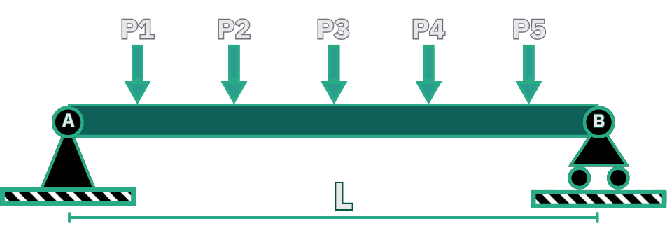
Application 2: Conveyor Roller Support Beam (Electromechanical)
A conveyor beam supports five equally spaced boxes during material handling operations.
🔧 Equivalent System Model
Given:
Beam length: L = 2000 mm
Support conditions: Simply supported at both ends
Load configuration: 5 boxes, each P = 400 N
Load spacing: 400 mm intervals (at x = 200, 600, 1000, 1400, 1800 mm)
Cross-section: Hollow rectangular steel 60×40×4 mm (I = 3.1×10⁶ mm⁴, c = 30 mm)
Material: Steel (σ_yield = 250 MPa)
Step 1: Calculate Reaction Forces
Click to reveal reaction force calculations
Sum of vertical forces (↑ positive):
✅
Sum of moments about A (counterclockwise positive):
✅
Calculate R_A:
✅
Verify by symmetry:
Since loads are symmetric about centerline (x = 1000 mm), reactions are equal: N ✅
Step 2: Construct Shear Force Diagram
Click to reveal shear force analysis
Method: Track cumulative loads from left support.
Key regions and jumps:
For 0 ≤ x < 200 mm: ✅
At x = 200 mm (first load):
Jump down by 400 N: V = 1000 - 400 = 600 N ✅
For 200 < x < 600 mm: ✅
At x = 600 mm (second load):
Jump down by 400 N: V = 600 - 400 = 200 N ✅
For 600 < x < 1000 mm: ✅
At x = 1000 mm (center load):
Jump down by 400 N: V = 200 - 400 = -200 N ✅
For 1000 < x < 1400 mm: ✅
At x = 1400 mm (fourth load):
Jump down by 400 N: V = -200 - 400 = -600 N ✅
For 1400 < x < 1800 mm: ✅
At x = 1800 mm (fifth load):
Jump down by 400 N: V = -600 - 400 = -1000 N ✅
For 1800 < x ≤ 2000 mm: ✅
Maximum shear force: |V_max| = 1000 N at both supports ✅
Step 3: Construct Bending Moment Diagram
Click to reveal bending moment analysis
Method: Integrate shear force or use equilibrium of cut sections.
For 0 ≤ x ≤ 200 mm:
For 200 ≤ x ≤ 600 mm:
For 600 ≤ x ≤ 1000 mm:
For 1000 ≤ x ≤ 1400 mm:
For 1400 ≤ x ≤ 1800 mm:
For 1800 ≤ x ≤ 2000 mm:
Maximum bending moment: M_max = 520,000 N·mm = 520 N·m at x = 1000 mm (center) ✅
Step 4: Critical Section Analysis
Click to reveal critical analysis and design recommendations
Maximum moment location:
Center (x = 1000 mm): M = 520 N·m ✅
Under loads (x = 600, 1400 mm): M = 440 N·m ✅
Critical location: Center of beam (midspan) despite no load at this point ✅
Engineering insight - Midspan vs Under-Load Comparison:
Why midspan is critical:
In simply supported beams with multiple point loads, moment builds up between loads
Midspan moment (520 N·m) > Under-load moment (440 N·m)
This occurs because the center experiences cumulative effect of loads on both sides
Design recommendation: Size beam based on midspan moment, not just load locations ✅
Practical implications:
Deflection will also be maximum at center
Lateral-torsional buckling check needed at center span
Consider intermediate supports if moment is excessive
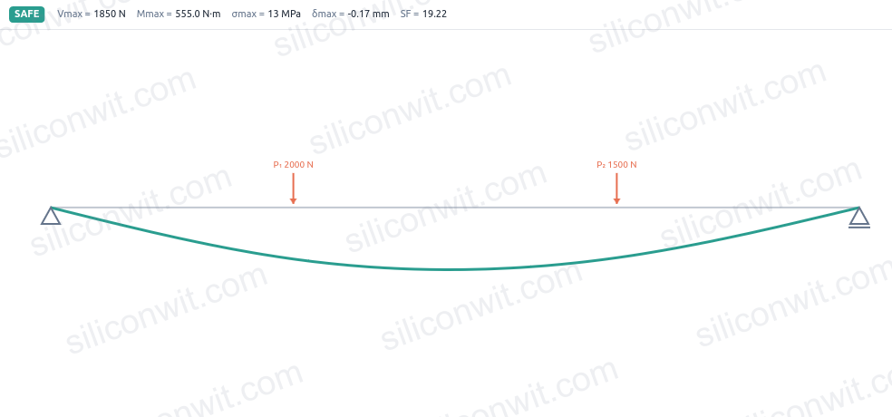
Application 3: Solar Tracker Arm (Electronics/Mechatronics)
A solar tracker support beam adjusts panel orientation to track the sun, experiencing combined self-weight, wind loading, and equipment forces.
🔧 Equivalent System Model
Given:
Total beam length: 3.0 m (2.5 m span + 0.5 m overhang)
Support A (pinned): at x = 0
Support B (roller): at x = 2.5 m
Uniformly distributed load: W = 300 N/m across entire length (panel weight + wind)
Point load at tip: P1 = 600 N at x = 3.0 m (clamp mechanism)
Cross-section: Structural steel I-beam (I = 6.8×10⁶ mm⁴, c = 40 mm)
Material: Structural steel (σ_yield = 250 MPa)
Step 1: Calculate Reaction Forces
Click to reveal reaction force calculations
Sum of vertical forces (↑ positive):
✅
Sum of moments about A (counterclockwise positive):
✅
Calculate R_A:
✅
Verification by moments about B:
Breaking down each term:
Moment from R_A: +240(2.5) = +600 N·m
Moment from UDL on span (0 to 2.5 m): -300(2.5)(1.25) = -937.5 N·m
Moment from UDL on overhang (2.5 to 3.0 m): +300(0.5)(0.25) = +37.5 N·m
Moment from P at tip: +600(0.5) = +300 N·m
✅
Step 2: Construct Shear Force Diagram
Click to reveal shear force analysis
Method: Track loads from left support, accounting for distributed load accumulation.
For 0 ≤ x ≤ 2.5 m (between supports):
For 2.5 < x ≤ 3.0 m (overhang region):
Key points:
At x = 0: V(0) = 240 N ✅
At x = 0.8 m: V(0.8) = 240 - 300(0.8) = 0 N ✅ (zero shear point)
Just before support B (x = 2.5⁻): V(2.5⁻) = 240 - 300(2.5) = -510 N ✅
Just after support B (x = 2.5⁺): V(2.5⁺) = -510 + 1260 = 750 N ✅
At tip before point load (x = 3.0⁻): V(3.0⁻) = 1500 - 300(3.0) = 600 N ✅
At tip after point load (x = 3.0⁺): V(3.0⁺) = 600 - 600 = 0 N ✅
Maximum shear forces:
Positive: V_max = 750 N just after support B ✅
Negative: V_min = -510 N just before support B ✅
Step 3: Construct Bending Moment Diagram
Click to reveal bending moment analysis
Method: Integrate shear force or use moment equilibrium of cut sections.
For 0 ≤ x ≤ 2.5 m:
With boundary condition M(0) = 0: C₁ = 0
For 2.5 < x ≤ 3.0 m:
With continuity at x = 2.5 m: M(2.5) = 240(2.5) - 150(2.5)² = -337.5 N·m
Key moment values:
At x = 0: M(0) = 0 N·m ✅
At x = 0.8 m (zero shear): M(0.8) = 240(0.8) - 150(0.8)² = 192 - 96 = 96 N·m ✅ ← Max positive
At x = 2.5 m (support B): M(2.5) = 240(2.5) - 150(2.5)² = 600 - 937.5 = -337.5 N·m ✅ ← Max negative
At x = 3.0 m (tip): M(3.0) = 1500(3.0) - 150(3.0)² - 3150 = 4500 - 1350 - 3150 = 0 N·m ✅
Maximum moments:
Positive: M_max = +96 N·m at x = 0.8 m ✅
Negative: M_min = -337.5 N·m at support B (x = 2.5 m) ✅
Step 4: Critical Section Analysis
Click to reveal critical bending stress assessment
Maximum moment comparison:
Positive moment: M_max = +96 N·m at x = 0.8 m ✅
Negative moment: |M_min| = 337.5 N·m at support B ✅
Critical location: Support B due to larger moment magnitude ✅
Engineering assessment - Positive vs Negative Moment Regions:
Why support B is most critical:
Negative moment (337.5 N·m) >> Positive moment (96 N·m)
Support experiences both high shear force and maximum negative moment
Design implication: Beam capacity controlled by support B, not midspan
Stress distribution at critical section:
Top fiber: Tension (negative moment causes beam to curve upward)
Bottom fiber: Compression
Design consideration: Check lateral-torsional buckling of compression flange
Practical design recommendations:
Reinforce support B region with stiffeners or larger section
Consider moment redistribution with semi-rigid connections
Check fatigue due to cyclic wind loading and tracking motion
Verify deflection limits especially in overhang region
Summary and Next Steps
In this lesson, you learned to:
Construct shear force diagrams using equilibrium (V = ΣF_y) and differential relationships (dV/dx = -w)
Build bending moment diagrams using integration (dM/dx = V) and moment equilibrium principles
Identify critical sections with maximum shear and moment values
Analyze cantilever, simply supported, and overhanging beam configurations
Determine reaction forces for fixed, pinned, and roller supports
Key Design Insights:
Cantilever beams: Maximum moment at fixed support
Simply supported beams: Maximum moment often at midspan
Overhanging beams: Critical section at intermediate support
Shear jumps at point loads, moment jumps at applied moments
Distributed loads create linear shear and parabolic moment curves
Critical Relationships:
Load-Shear: dV/dx = -w(x)
Shear-Moment: dM/dx = V(x)
Maximum moment: Occurs where V(x) = 0
Coming Next: In Lesson 2.2, we’ll calculate bending stresses using the flexure formula σ = My/I to determine if beam designs can safely support operational loads.


Comments