Lab 1: Shear Force and Bending Moment
Application: Robotic Arm Cantilever Analysis
- Calculate reaction forces and internal loads
- Generate SFD/BMD using Python
- Create 3D visualization in FreeCAD
- Duration: 1 week
Hand calculations tell you the stress at a single point under idealized loading. Real structures have complex geometry, multiple load paths, and boundary conditions that are difficult to capture analytically. Finite element analysis handles that complexity, but trusting its output blindly is dangerous: a wrong mesh, a misapplied boundary condition, or a misunderstood result can produce numbers that look plausible but are wrong. The only reliable check is to solve a simplified version analytically, compare it to FEA, and understand where and why they diverge. These three progressive labs do exactly that for a robotic arm cantilever, a 3D printer gantry rail, and a drone arm under combined loading.
This laboratory series provides comprehensive training in structural analysis methods essential for modern engineering practice. You will analyze real engineering components using both analytical methods (Python) and finite element analysis (FreeCAD), developing skills directly applicable to mechatronics, automation, and structural design.
Modern engineering requires proficiency in multiple analysis methods: hand calculations for understanding fundamentals, programming for automation and parametric studies, and finite element methods for complex geometries and loading conditions. This laboratory series develops all three competencies through practical applications.
Core Laboratory Skills:
Lab 1: Shear Force and Bending Moment
Application: Robotic Arm Cantilever Analysis
Lab 2: Bending Stresses and FEM
Application: 3D Printer Gantry Rail Design
Lab 3: Combined Loading Analysis
Application: Drone Arm Multi-Axis Loading
All submitted files must follow a strict naming convention to ensure proper organization and grading.
📁 Standard File Naming Format
Format: E022-01-XXXX-YYYY-LabN-Type.extension
Components:
E022-01 = Course codeXXXX = Your 4-digit registration number (e.g., 1234)YYYY = Registration year (e.g., 2023)LabN = Lab number (Lab1, Lab2, or Lab3)Type = File type descriptor.extension = Appropriate file extensionExample: E022-01-1234-2023-Lab1-Model.glb
📋 Required File Types and Naming
For Each Lab, Submit:
3D Model (GLB format)
E022-01-XXXX-YYYY-LabN-Model.glbTechnical Drawing (PDF format)
E022-01-XXXX-YYYY-LabN-Drawing.pdfRendered Images (PNG format)
E022-01-XXXX-YYYY-LabN-Isometric.pngE022-01-XXXX-YYYY-LabN-SideView.pngPython Script (PY format)
E022-01-XXXX-YYYY-LabN-Analysis.pyAnalysis Plots (PNG format)
E022-01-XXXX-YYYY-Lab1-SFD-BMD.pngE022-01-XXXX-YYYY-Lab2-StressAnalysis.pngE022-01-XXXX-YYYY-Lab2-Convergence.pngE022-01-XXXX-YYYY-Lab3-MohrsCircle.pngE022-01-XXXX-YYYY-Lab3-Optimization.pngHand Calculations (PDF format)
E022-01-XXXX-YYYY-LabN-Calculations.pdfTechnical Report (PDF format)
E022-01-XXXX-YYYY-LabN-Report.pdf📦 Submission Package Structure
Create a folder named: E022-01-XXXX-YYYY-LabN (the group leader’s Reg. No.)
Inside the folder, organize files:
E022-01-1234-2023-Lab1/├── E022-01-1234-2023-Lab1-Model.glb├── E022-01-1234-2023-Lab1-Drawing.pdf├── E022-01-1234-2023-Lab1-Isometric.png├── E022-01-1234-2023-Lab1-SideView.png├── E022-01-1234-2023-Lab1-Analysis.py├── E022-01-1234-2023-Lab1-SFD-BMD.png├── E022-01-1234-2023-Lab1-Calculations.pdf└── E022-01-1234-2023-Lab1-Report.pdfCompress to ZIP: E022-01-XXXX-YYYY-LabN.zip
Submit to the instructor before deadline
Lab Duration: 1 week
By the end of this laboratory, you will be able to:
You are designing a 6-DOF industrial robotic manipulator for material handling operations. The forearm segment connects the wrist joint to the gripper and must support the payload while maintaining sufficient rigidity to ensure positioning accuracy. The arm is modeled as a cantilever beam fixed at the elbow joint.
Design Challenge: The beam must safely support operational loads while minimizing weight to reduce motor torque requirements and improve dynamic response. Excessive deflection would compromise positioning accuracy, while insufficient strength could lead to structural failure.
📋 Robotic Arm Specifications
Geometry:
Loading:
Material:
Support Configuration:
Critical Question: What are the maximum shear force and bending moment for this robotic arm, and where do they occur?
Before writing any code, develop fundamental understanding through hand calculations.
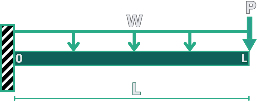
Draw Free Body Diagram (Equivalent System Model)
Sketch the beam showing:
Calculate Reaction Forces
For cantilever beam with end load, apply equilibrium:
Vertical force equilibrium (↑ positive):
Moment equilibrium about fixed support (counterclockwise positive):
Determine Shear Force Distribution
For cantilever with end load, shear force is constant along length:
(Negative because load creates downward shear on right side of any cut)
At free end after load point: V = 0 N
Determine Bending Moment Distribution
Bending moment varies linearly from support to free end:
At key points:
Calculate Maximum Bending Stress
Use the flexure formula:
Calculate Safety Factor
Engineering Insight: This safety factor of 4.4 is appropriate for robotic applications. In practice, SF = 3-5 is typical for robotics where dynamic loads, impact, and reliability are important considerations. This design balances safety with reasonable material usage.
Now automate this analysis using Python for rapid design iteration and parametric studies.
Install required libraries:
pip install numpy matplotlib scipy pandasimport numpy as npimport matplotlib.pyplot as plt
# ===== PROBLEM PARAMETERS =====# GeometryL = 500 # Beam length in mmb = 60 # Width in mmh = 20 # Height in mm
# LoadingP = 500 # Point load in N
# Materialsigma_yield = 275 # Yield strength in MPa
# Section propertiesI = (b * h**3) / 12 # Moment of inertia in mm^4c = h / 2 # Distance to outer fiber in mm
print(f'Moment of Inertia: {I:.2e} mm^4')print(f'Distance to outer fiber: {c:.1f} mm')
# ===== ANALYSIS =====# Create position array (0 to L)x = np.linspace(0, L, 100)
# Shear force (constant for cantilever with end load)V = -np.ones_like(x) * P # Negative shear throughout
# Bending moment (linear variation)M = -P * (L - x) # Negative indicates tension on top fiber
# Find maximum valuesV_max = np.max(np.abs(V))M_max = np.max(np.abs(M))M_max_location = x[np.argmax(np.abs(M))]
# Calculate maximum bending stresssigma_max = (M_max * c) / I # in N/mm^2 = MPa
# Safety factorSF = sigma_yield / sigma_max
# ===== PRINT RESULTS =====print('\n===== ANALYSIS RESULTS =====')print(f'Maximum Shear Force: {V_max:.1f} N')print(f'Maximum Bending Moment: {M_max:.1f} N·mm = {M_max/1000:.2f} N·m')print(f'Location of M_max: {M_max_location:.1f} mm from fixed end')print(f'Maximum Bending Stress: {sigma_max:.2f} MPa')print(f'Safety Factor: {SF:.2f}')
# ===== CREATE PLOTS =====fig, (ax1, ax2) = plt.subplots(2, 1, figsize=(10, 8))
# Shear Force Diagramax1.plot(x, V, 'b-', linewidth=2, label='Shear Force')ax1.axhline(y=0, color='k', linestyle='--', linewidth=0.5)ax1.fill_between(x, 0, V, alpha=0.3, color='blue')ax1.set_xlabel('Position along beam (mm)', fontsize=12)ax1.set_ylabel('Shear Force (N)', fontsize=12)ax1.set_title('Shear Force Diagram - Robotic Arm Cantilever', fontsize=14, fontweight='bold')ax1.grid(True, alpha=0.3)ax1.legend()
# Bending Moment Diagramax2.plot(x, M/1000, 'r-', linewidth=2, label='Bending Moment')ax2.axhline(y=0, color='k', linestyle='--', linewidth=0.5)ax2.fill_between(x, 0, M/1000, alpha=0.3, color='red')ax2.set_xlabel('Position along beam (mm)', fontsize=12)ax2.set_ylabel('Bending Moment (N·m)', fontsize=12)ax2.set_title('Bending Moment Diagram - Robotic Arm Cantilever', fontsize=14, fontweight='bold')ax2.grid(True, alpha=0.3)ax2.legend()
plt.tight_layout()plt.savefig('SFD_BMD_RoboticArm.png', dpi=300, bbox_inches='tight')plt.show()
print('\nPlots saved as SFD_BMD_RoboticArm.png')Expected Console Output:
Moment of Inertia: 4.00e+04 mm^4Distance to outer fiber: 10.0 mm
===== ANALYSIS RESULTS =====Maximum Shear Force: 500.0 NMaximum Bending Moment: 250000.0 N·mm = 250.00 N·mLocation of M_max: 0.0 mm from fixed endMaximum Bending Stress: 62.50 MPaSafety Factor: 4.40Your Plots Should Show:
Shear Force Diagram:
Bending Moment Diagram:
Create a 3D model of the robotic arm in FreeCAD to visualize the component and understand its geometry.
Beam Geometry and Orientation:
Coordinate System (FreeCAD Standard):┌─────────────────────────────────────────────────┐│ X-axis: Beam LENGTH (500 mm) → extends left-right│ Y-axis: Beam WIDTH (60 mm) → extends front-back│ Z-axis: Beam HEIGHT (20 mm) → extends up-down││ Cross-section: 60 mm (Y) × 20 mm (Z) rectangle│ Extrusion: Along X-axis for 500 mm││ Load: P = 500 N pointing DOWN (-Z direction)│ at x = 500 mm (free end, right side)││ Support: Fixed at x = 0 mm (left side)└─────────────────────────────────────────────────┘Create Basic Beam Model
Draw Rectangular Cross-Section (60 mm wide × 20 mm tall)
Extrude Beam Along Length (500 mm)
Add Material Properties
Add Load Visualization (Arrow Pointing Downward)
Add Fixed Support Visualization
Create Technical Drawing (TechDraw Workbench)
Add Multiple Views:
Add Dimensions:
Add Annotations:
Export Drawing:
E022-01-XXXX-YYYY-Lab1-Drawing.pdfExport 3D Model and Images
Set Isometric View:
Take Screenshots:
E022-01-XXXX-YYYY-Lab1-Isometric.png
E022-01-XXXX-YYYY-Lab1-SideView.png
Export 3D Model (GLB for Web):
.gltf to .glb before saving
E022-01-XXXX-YYYY-Lab1-Model.gltfE022-01-XXXX-YYYY-Lab1-Model.glb.glb file to confirm it displays correctly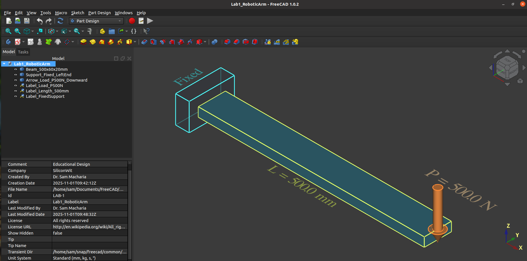
Example FreeCAD model showing beam, fixed support, and load arrow
Submit according to the File Naming and Submission Standards above.
Required Files:
3D Model - E022-01-XXXX-YYYY-Lab1-Model.glb
Technical Drawing - E022-01-XXXX-YYYY-Lab1-Drawing.pdf
Rendered Images
E022-01-XXXX-YYYY-Lab1-Isometric.png (isometric view showing load and support)E022-01-XXXX-YYYY-Lab1-SideView.png (side elevation showing beam dimensions)Python Script - E022-01-XXXX-YYYY-Lab1-Analysis.py
Analysis Plot - E022-01-XXXX-YYYY-Lab1-SFD-BMD.png
Hand Calculations - E022-01-XXXX-YYYY-Lab1-Calculations.pdf
Technical Report - E022-01-XXXX-YYYY-Lab1-Report.pdf (2-3 pages)
Submission: Compress all files into E022-01-XXXX-YYYY-Lab1.zip and submit to the instructor.
Lab Duration: 1 week
By the end of this laboratory, you will be able to:
Desktop 3D printers use a horizontal rail (gantry) that supports the print head as it moves back and forth during the additive manufacturing process. The rail must be stiff enough to prevent deflection during printing, which would cause layer misalignment and poor print quality. The print head weight creates a moving concentrated load that varies in position during operation.
Design Challenge: The gantry must maintain positioning accuracy within ±0.05 mm while minimizing weight to enable faster print speeds. Understanding where maximum stresses occur is critical for optimizing the rail cross-section and selecting appropriate materials.
📋 3D Printer Gantry Specifications
Geometry:
Loading:
Material:
Support Configuration:
Critical Questions:
First, determine the critical load position and maximum stress analytically.
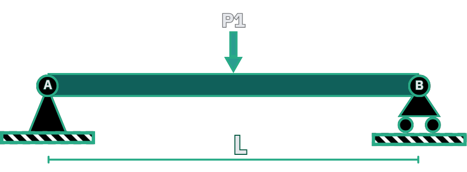
For a simply supported beam with point load P at distance ‘a’ from left support:
Left reaction:
Right reaction:
Bending moment under load:
To find position ‘a’ that gives absolute maximum moment, differentiate and set to zero:
Therefore: Maximum bending moment occurs when load is at midspan (a = L/2 = 400 mm)
Calculate Maximum Moment
With load at midspan (a = 400 mm):
Calculate Maximum Bending Stress
Apply flexure formula:
Calculate Safety Factor
Engineering Assessment
This extremely high static safety factor indicates the rail is over-designed for static loading. However, 3D printers involve:
These dynamic effects can create stress amplification factors of 2-5×. A high static SF provides margin for dynamic effects and ensures long service life.
Create Python code to analyze stress at multiple load positions and generate visualization plots.
import numpy as npimport matplotlib.pyplot as plt
# ===== PROBLEM PARAMETERS =====# GeometryL = 800  # Rail length in mmOD = 30  # Outer diameter in mmt = 3  # Wall thickness in mmID = OD - 2*t  # Inner diameter in mm
# LoadingP = 200  # Print head weight in N
# Materialsigma_yield = 275  # Yield strength in MPaE = 70000  # Young's modulus in MPa
# Section properties (hollow circular)I = (np.pi / 64) * (OD**4 - ID**4)  # Moment of inertia in mm^4c = OD / 2  # Distance to outer fiber in mm
print(f'Moment of Inertia: {I:.2e} mm^4')print(f'Distance to outer fiber: {c:.1f} mm')
# ===== PARAMETRIC ANALYSIS =====# Analyze load at multiple positionsa_positions = np.linspace(0, L, 200)  # Load positions
# Calculate moment at each positionM_at_load = P * a_positions * (L - a_positions) / L
# Calculate stress at each positionsigma = (M_at_load * c) / I
# Find maximum valuesa_critical = a_positions[np.argmax(sigma)]M_max = np.max(M_at_load)sigma_max = np.max(sigma)SF = sigma_yield / sigma_max
# ===== PRINT RESULTS =====print('\n===== ANALYSIS RESULTS =====')print(f'Critical load position: {a_critical:.1f} mm from left support')print(f'Maximum bending moment: {M_max:.1f} N·mm = {M_max/1000:.2f} N·m')print(f'Maximum bending stress: {sigma_max:.3f} MPa')print(f'Safety factor: {SF:.1f}')
# ===== CREATE PLOTS =====fig, (ax1, ax2) = plt.subplots(2, 1, figsize=(10, 8))
# Bending Moment vs Load Positionax1.plot(a_positions, M_at_load/1000, 'b-', linewidth=2)ax1.axvline(x=a_critical, color='r', linestyle='--', linewidth=1, label=f'Critical position: {a_critical:.0f} mm')ax1.axhline(y=M_max/1000, color='gray', linestyle=':', linewidth=1)ax1.set_xlabel('Load Position (mm)', fontsize=12)ax1.set_ylabel('Bending Moment (N·m)', fontsize=12)ax1.set_title('Bending Moment vs Print Head Position', fontsize=14, fontweight='bold')ax1.grid(True, alpha=0.3)ax1.legend()
# Bending Stress vs Load Positionax2.plot(a_positions, sigma, 'r-', linewidth=2)ax2.axvline(x=a_critical, color='b', linestyle='--', linewidth=1, label=f'Max stress: {sigma_max:.3f} MPa')ax2.axhline(y=sigma_max, color='gray', linestyle=':', linewidth=1)ax2.axhline(y=sigma_yield, color='orange', linestyle='--', linewidth=2, label=f'Yield strength: {sigma_yield} MPa')ax2.set_xlabel('Load Position (mm)', fontsize=12)ax2.set_ylabel('Maximum Bending Stress (MPa)', fontsize=12)ax2.set_title('Bending Stress vs Print Head Position', fontsize=14, fontweight='bold')ax2.grid(True, alpha=0.3)ax2.legend()
plt.tight_layout()plt.savefig('GantryRail_Stress_Analysis.png', dpi=300, bbox_inches='tight')plt.show()
print('\nPlots saved as GantryRail_Stress_Analysis.png')
Expected Results:
Now validate the analytical solution using finite element analysis.
Create 3D Model of Hollow Circular Tube
Switch to FEM Workbench
Add Material
Apply Boundary Conditions - Left Support (Pin)
Apply Boundary Conditions - Right Support (Roller)
Apply Load at Midspan
Create Mesh
Run Solver
View Results
Compare with Analytical Solution
Verify that your FEM results are mesh-independent by refining the mesh.
🔬 Mesh Convergence Procedure
Why Convergence Studies Matter:
FEM approximates reality by dividing continuous structure into discrete elements. Coarse meshes give approximate results; finer meshes converge toward exact solution. Engineers must verify their mesh is sufficiently refined.
Procedure:
Convergence Criterion:
Solution has converged when refining mesh changes result by less than 2-5%.
Create Python script to analyze convergence:
import matplotlib.pyplot as plt
# Mesh convergence data (fill in from your FEM runs)element_sizes = [20, 10, 5]  # mmnum_elements = []  # Record from FreeCADmax_stress_fem = []  # Record from FEM results (MPa)
# Analytical solution for comparisonsigma_analytical = 0.682  # MPa
# Calculate percent errorpercent_error = [(abs(s - sigma_analytical) / sigma_analytical * 100) for s in max_stress_fem]
# Plot convergencefig, (ax1, ax2) = plt.subplots(1, 2, figsize=(12, 5))
# Stress vs number of elementsax1.plot(num_elements, max_stress_fem, 'bo-', linewidth=2, markersize=8, label='FEM Results')ax1.axhline(y=sigma_analytical, color='r', linestyle='--', linewidth=2, label='Analytical Solution')ax1.set_xlabel('Number of Elements', fontsize=12)ax1.set_ylabel('Maximum Stress (MPa)', fontsize=12)ax1.set_title('Mesh Convergence Study', fontsize=14, fontweight='bold')ax1.grid(True, alpha=0.3)ax1.legend()
# Percent error vs number of elementsax2.plot(num_elements, percent_error, 'ro-', linewidth=2, markersize=8)ax2.axhline(y=5, color='gray', linestyle='--', linewidth=1, label='5% error threshold')ax2.set_xlabel('Number of Elements', fontsize=12)ax2.set_ylabel('Percent Error (%)', fontsize=12)ax2.set_title('FEM Error vs Mesh Refinement', fontsize=14, fontweight='bold')ax2.grid(True, alpha=0.3)ax2.legend()
plt.tight_layout()plt.savefig('Mesh_Convergence_Study.png', dpi=300, bbox_inches='tight')plt.show()Submit according to the File Naming and Submission Standards above.
Required Files:
3D FEM Model - E022-01-XXXX-YYYY-Lab2-Model.glb
Technical Drawing - E022-01-XXXX-YYYY-Lab2-Drawing.pdf
Rendered Images
E022-01-XXXX-YYYY-Lab2-Isometric.png (FEM stress contours visible)E022-01-XXXX-YYYY-Lab2-SideView.png (showing support conditions and load position)Python Scripts
E022-01-XXXX-YYYY-Lab2-Analysis.py (parametric stress analysis)E022-01-XXXX-YYYY-Lab2-Convergence.py (mesh convergence study)Analysis Plots
E022-01-XXXX-YYYY-Lab2-StressAnalysis.png (stress vs load position, moment vs load position)E022-01-XXXX-YYYY-Lab2-Convergence.png (convergence plot showing stress vs element count)Hand Calculations - E022-01-XXXX-YYYY-Lab2-Calculations.pdf
Technical Report - E022-01-XXXX-YYYY-Lab2-Report.pdf (3-4 pages)
Submission: Compress all files into E022-01-XXXX-YYYY-Lab2.zip and submit to the instructor.
Lab Duration: 1 week
By the end of this laboratory, you will be able to:
Quadcopter drones use four motor arms extending from the central body to support the motors and propellers. Each arm experiences complex loading: vertical thrust forces from motors, aerodynamic drag creating bending, and gyroscopic moments from spinning propellers creating torsion. The arms must withstand these combined loads while minimizing weight for maximum flight time.
Design Challenge: Optimize the arm cross-section to achieve a safety factor of 3.0 under combined loading while minimizing mass. Every gram saved increases flight time, but insufficient strength leads to catastrophic failure during flight.
📋 Drone Arm Specifications
Geometry:
Loading:
Material:
Support Configuration:
Critical Questions:
Analyze each loading component separately, then combine using superposition.
Analyze Bending from Vertical Thrust
Vertical load P = 50 N creates bending moment at fixed end:
Maximum bending stress (at top and bottom of section):
(Tension on bottom, compression on top)
Analyze Bending from Horizontal Drag
Horizontal load F = 8 N creates bending in orthogonal plane:
Maximum bending stress (at sides of section):
Analyze Torsion from Gyroscopic Moment
Applied torque T = 2 N·m = 2000 N·mm creates shear stress:
Identify Critical Point
The critical point is at the fixed end, at the location where bending stresses from both planes combine constructively. For circular tube, consider point at 45° where both bending components contribute:
Calculate Principal Stresses
For plane stress state (σ_x, τ_xy):
Apply Von Mises Failure Criterion
For ductile materials (conservative for composites):
Safety factor:
Apply Maximum Stress Criterion (More Appropriate for Composites)
For brittle composites, compare maximum stress to strength:
Governing safety factor: 13.5
Engineering Assessment: The safety factor exceeds 10, indicating significant over-design. This provides margin for:
However, weight reduction could increase flight time. Target SF = 3-4 would be more appropriate.
Automate combined stress analysis and visualize stress state using Mohr’s circle.
import numpy as npimport matplotlib.pyplot as plt
# ===== PROBLEM PARAMETERS =====# GeometryL = 250  # Arm length in mmOD = 20  # Outer diameter in mmID = 16  # Inner diameter in mmr_outer = OD / 2r_inner = ID / 2
# LoadingP_vertical = 50  # NF_horizontal = 8  # NT_torque = 2000  # N·mm
# Material (carbon fiber)sigma_tensile = 600  # MPasigma_compressive = 500  # MPatau_ultimate = 70  # MPa
# Section propertiesJ = (np.pi / 32) * (OD**4 - ID**4)  # Polar momentI = (np.pi / 64) * (OD**4 - ID**4)  # Moment of inertia
print(f'Polar Moment of Inertia: {J:.1f} mm^4')print(f'Moment of Inertia: {I:.1f} mm^4')
# ===== STRESS ANALYSIS =====# Bending momentsM_vertical = P_vertical * LM_horizontal = F_horizontal * L
# Bending stresses at critical pointsigma_vertical = (M_vertical * r_outer) / Isigma_horizontal = (M_horizontal * r_outer) / I
# Combined bending stress (vector sum for worst case)sigma_x = np.sqrt(sigma_vertical**2 + sigma_horizontal**2)
# Torsional shear stresstau_xy = (T_torque * r_outer) / J
print('\n===== STRESS COMPONENTS =====')print(f'Bending stress (vertical load): {sigma_vertical:.2f} MPa')print(f'Bending stress (horizontal load): {sigma_horizontal:.2f} MPa')print(f'Combined bending stress: {sigma_x:.2f} MPa')print(f'Torsional shear stress: {tau_xy:.2f} MPa')
# ===== PRINCIPAL STRESSES =====# For plane stress: sigma_x, tau_xysigma_avg = sigma_x / 2R = np.sqrt((sigma_x/2)**2 + tau_xy**2)
sigma_1 = sigma_avg + Rsigma_2 = sigma_avg - Rsigma_3 = 0  # plane stress
print('\n===== PRINCIPAL STRESSES =====')print(f'σ₁ (maximum principal): {sigma_1:.2f} MPa')print(f'σ₂ (minimum principal): {sigma_2:.2f} MPa')print(f'σ₃ (out-of-plane): {sigma_3:.2f} MPa')
# ===== FAILURE CRITERIA =====# Von Mises stresssigma_vm = np.sqrt(((sigma_1-sigma_2)**2 + (sigma_2-sigma_3)**2 + (sigma_3-sigma_1)**2) / 2)
# Tresca (maximum shear stress)tau_max = (sigma_1 - sigma_2) / 2
# Safety factorsSF_von_mises = sigma_compressive / sigma_vmSF_max_stress_tensile = sigma_tensile / sigma_1SF_max_stress_shear = tau_ultimate / tau_max
print('\n===== FAILURE ANALYSIS =====')print(f'Von Mises equivalent stress: {sigma_vm:.2f} MPa')print(f'Maximum shear stress (Tresca): {tau_max:.2f} MPa')print(f'\nSafety Factors:')print(f'  Von Mises criterion: {SF_von_mises:.2f}')print(f'  Maximum stress (tension): {SF_max_stress_tensile:.2f}')print(f'  Maximum shear: {SF_max_stress_shear:.2f}')print(f'\nGoverning safety factor: {min(SF_von_mises, SF_max_stress_tensile, SF_max_stress_shear):.2f}')
# ===== MOHR'S CIRCLE VISUALIZATION =====fig, ax = plt.subplots(figsize=(10, 8))
# Circle parameterscenter = sigma_avgradius = R
# Draw circletheta = np.linspace(0, 2*np.pi, 100)circle_x = center + radius * np.cos(theta)circle_y = radius * np.sin(theta)
ax.plot(circle_x, circle_y, 'b-', linewidth=2, label="Mohr's Circle")
# Draw axesax.axhline(y=0, color='k', linestyle='-', linewidth=0.5)ax.axvline(x=0, color='k', linestyle='-', linewidth=0.5)
# Plot principal stressesax.plot([sigma_1, sigma_2], [0, 0], 'ro', markersize=10, label='Principal Stresses')ax.text(sigma_1, 2, f'σ₁ = {sigma_1:.1f} MPa', fontsize=11, ha='center')ax.text(sigma_2, -2, f'σ₂ = {sigma_2:.1f} MPa', fontsize=11, ha='center')
# Plot original stress stateax.plot([sigma_x, 0], [tau_xy, -tau_xy], 'gs', markersize=8, label='Original State')
# Draw line connecting original state pointsax.plot([sigma_x, 0], [tau_xy, -tau_xy], 'g--', linewidth=1)
# Labels and formattingax.set_xlabel('Normal Stress σ (MPa)', fontsize=13)ax.set_ylabel('Shear Stress τ (MPa)', fontsize=13)ax.set_title("Mohr's Circle - Drone Arm Combined Loading", fontsize=15, fontweight='bold')ax.grid(True, alpha=0.3)ax.legend(fontsize=11)ax.axis('equal')
plt.tight_layout()plt.savefig('Mohrs_Circle_DroneArm.png', dpi=300, bbox_inches='tight')plt.show()
print("\nMohr's circle saved as Mohrs_Circle_DroneArm.png")Validate analytical results using FreeCAD FEM with multiple load types.
Create Circular Tube Model
Setup FEM Analysis
Apply Fixed Constraint
Apply Vertical Force
Apply Horizontal Force
Apply Torque
Mesh and Solve
Analyze Results
View Principal Stresses
Use Python to perform parametric study for weight optimization.
import numpy as npimport matplotlib.pyplot as plt
# Design constraintsSF_target = 3.0  # Target safety factorL = 250  # Length fixedsigma_allowable = sigma_compressive / SF_target  # 500/3 = 166.7 MPa
# Vary tube dimensionsOD_range = np.linspace(12, 24, 30)  # Outer diameter rangethickness = 2  # Fix wall thickness at 2mmID_range = OD_range - 2*thickness
# Material densityrho = 1.6e-6  # kg/mm^3 (carbon fiber)
masses = []safety_factors = []
for OD, ID in zip(OD_range, ID_range):    r_outer = OD / 2    r_inner = ID / 2
    # Section properties    J = (np.pi / 32) * (OD**4 - ID**4)    I = (np.pi / 64) * (OD**4 - ID**4)
    # Stress analysis (same loading)    M_v = P_vertical * L    M_h = F_horizontal * L    sigma_v = (M_v * r_outer) / I    sigma_h = (M_h * r_outer) / I    sigma_x = np.sqrt(sigma_v**2 + sigma_h**2)    tau_xy = (T_torque * r_outer) / J
    # Principal stress    R = np.sqrt((sigma_x/2)**2 + tau_xy**2)    sigma_1 = sigma_x/2 + R
    # Von Mises    sigma_vm = np.sqrt(sigma_1**2 + 3*tau_xy**2)  # Simplified for comparison
    # Safety factor    SF = sigma_compressive / sigma_vm    safety_factors.append(SF)
    # Mass calculation    volume = np.pi * (r_outer**2 - r_inner**2) * L    mass = volume * rho * 1000  # Convert to grams    masses.append(mass)
# Find optimal designoptimal_idx = np.argmin([abs(sf - SF_target) for sf in safety_factors])optimal_OD = OD_range[optimal_idx]optimal_mass = masses[optimal_idx]optimal_SF = safety_factors[optimal_idx]
# Plottingfig, (ax1, ax2) = plt.subplots(1, 2, figsize=(14, 5))
# Mass vs Outer Diameterax1.plot(OD_range, masses, 'b-', linewidth=2)ax1.plot(optimal_OD, optimal_mass, 'ro', markersize=12, label=f'Optimal: OD={optimal_OD:.1f}mm, m={optimal_mass:.1f}g')ax1.set_xlabel('Outer Diameter (mm)', fontsize=12)ax1.set_ylabel('Mass (grams)', fontsize=12)ax1.set_title('Arm Mass vs Tube Diameter', fontsize=14, fontweight='bold')ax1.grid(True, alpha=0.3)ax1.legend()
# Safety Factor vs Outer Diameterax2.plot(OD_range, safety_factors, 'r-', linewidth=2)ax2.axhline(y=SF_target, color='g', linestyle='--', linewidth=2, label=f'Target SF = {SF_target}')ax2.plot(optimal_OD, optimal_SF, 'ro', markersize=12, label=f'Optimal: SF={optimal_SF:.2f}')ax2.set_xlabel('Outer Diameter (mm)', fontsize=12)ax2.set_ylabel('Safety Factor', fontsize=12)ax2.set_title('Safety Factor vs Tube Diameter', fontsize=14, fontweight='bold')ax2.grid(True, alpha=0.3)ax2.legend()
plt.tight_layout()plt.savefig('Design_Optimization_Study.png', dpi=300, bbox_inches='tight')plt.show()
print('\n===== OPTIMIZATION RESULTS =====')print(f'Optimal outer diameter: {optimal_OD:.1f} mm')print(f'Optimal mass per arm: {optimal_mass:.1f} grams')print(f'Safety factor achieved: {optimal_SF:.2f}')print(f'\nOriginal design: OD=20mm, mass={masses[list(OD_range).index(20)]:.1f}g')print(f'Mass savings: {masses[list(OD_range).index(20)] - optimal_mass:.1f}g ({(masses[list(OD_range).index(20)] - optimal_mass)/masses[list(OD_range).index(20)]*100:.1f}%)')print(f'Total savings for 4 arms: {4*(masses[list(OD_range).index(20)] - optimal_mass):.1f}g')Submit according to the File Naming and Submission Standards above.
Required Files:
3D FEM Model - E022-01-XXXX-YYYY-Lab3-Model.glb
Technical Drawing - E022-01-XXXX-YYYY-Lab3-Drawing.pdf
Rendered Images
E022-01-XXXX-YYYY-Lab3-Isometric.png (FEM von Mises stress contours)E022-01-XXXX-YYYY-Lab3-SideView.png (principal stress visualization)Python Scripts
E022-01-XXXX-YYYY-Lab3-Analysis.py (combined stress and Mohr’s circle analysis)E022-01-XXXX-YYYY-Lab3-Optimization.py (design optimization study)Analysis Plots
E022-01-XXXX-YYYY-Lab3-MohrsCircle.png (Mohr’s circle with principal stresses labeled)E022-01-XXXX-YYYY-Lab3-Optimization.png (mass vs safety factor, optimal design point)Hand Calculations - E022-01-XXXX-YYYY-Lab3-Calculations.pdf
Comprehensive Technical Report - E022-01-XXXX-YYYY-Lab3-Report.pdf (5-6 pages)
Submission: Compress all files into E022-01-XXXX-YYYY-Lab3.zip and submit to the instructor.
To ensure independent work while maintaining collaborative learning, each group receives slightly different parameters. Your instructor will assign one of these parameter sets to your group.
Lab 1: Robotic Arm - Group Parameters
| Group | Length (mm) | Load (N) | Width (mm) | Height (mm) |
|---|---|---|---|---|
| 1 | 501 | 542 | 60 | 20 |
| 2 | 464 | 521 | 60 | 20 |
| 3 | 510 | 470 | 60 | 20 |
| 4 | 532 | 536 | 60 | 20 |
| 5 | 524 | 524 | 60 | 20 |
| 6 | 537 | 549 | 60 | 20 |
| 7 | 473 | 452 | 60 | 20 |
| 8 | 471 | 502 | 60 | 20 |
| 9 | 451 | 537 | 60 | 20 |
| 10 | 479 | 487 | 60 | 20 |
| 11 | 451 | 513 | 60 | 20 |
| 12 | 509 | 470 | 60 | 20 |
| 13 | 482 | 525 | 60 | 20 |
| 14 | 507 | 471 | 60 | 20 |
| 15 | 538 | 498 | 60 | 20 |
| 16 | 540 | 508 | 60 | 20 |
| 17 | 491 | 541 | 60 | 20 |
| 18 | 509 | 529 | 60 | 20 |
| 19 | 464 | 511 | 60 | 20 |
| 20 | 511 | 496 | 60 | 20 |
Note: Cross-section dimensions (60mm × 20mm) remain constant for all groups. Only beam length and load vary.
Lab 2: 3D Printer Gantry - Group Parameters
| Group | Length (mm) | Load (N) | Outer Dia (mm) | Wall Thickness (mm) |
|---|---|---|---|---|
| 1 | 818 | 180 | 30 | 3 |
| 2 | 799 | 201 | 30 | 3 |
| 3 | 808 | 196 | 30 | 3 |
| 4 | 801 | 197 | 30 | 3 |
| 5 | 809 | 207 | 30 | 3 |
| 6 | 816 | 210 | 30 | 3 |
| 7 | 837 | 180 | 30 | 3 |
| 8 | 785 | 191 | 30 | 3 |
| 9 | 839 | 181 | 30 | 3 |
| 10 | 784 | 191 | 30 | 3 |
| 11 | 816 | 215 | 30 | 3 |
| 12 | 754 | 216 | 30 | 3 |
| 13 | 826 | 204 | 30 | 3 |
| 14 | 797 | 212 | 30 | 3 |
| 15 | 824 | 189 | 30 | 3 |
| 16 | 784 | 184 | 30 | 3 |
| 17 | 778 | 189 | 30 | 3 |
| 18 | 757 | 200 | 30 | 3 |
| 19 | 797 | 220 | 30 | 3 |
| 20 | 803 | 212 | 30 | 3 |
Note: Tube dimensions (OD=30mm, wall=3mm) remain constant. Only beam length and load vary.
Lab 3: Drone Arm - Group Parameters
| Group | Length (mm) | P_vert (N) | F_horiz (N) | Torque (N·mm) | OD (mm) | ID (mm) |
|---|---|---|---|---|---|---|
| 1 | 200 | 30 | 5 | 1073 | 16 | 12 |
| 2 | 183 | 27 | 4 | 1031 | 16 | 12 |
| 3 | 203 | 33 | 5 | 1095 | 16 | 12 |
| 4 | 187 | 30 | 6 | 1009 | 16 | 12 |
| 5 | 216 | 32 | 5 | 901 | 16 | 12 |
| 6 | 194 | 27 | 4 | 993 | 16 | 12 |
| 7 | 201 | 30 | 4 | 974 | 16 | 12 |
| 8 | 216 | 28 | 6 | 972 | 16 | 12 |
| 9 | 209 | 32 | 4 | 974 | 16 | 12 |
| 10 | 202 | 29 | 6 | 1044 | 16 | 12 |
| 11 | 188 | 30 | 6 | 918 | 16 | 12 |
| 12 | 208 | 32 | 5 | 963 | 16 | 12 |
| 13 | 192 | 29 | 5 | 966 | 16 | 12 |
| 14 | 189 | 27 | 5 | 908 | 16 | 12 |
| 15 | 216 | 29 | 6 | 1023 | 16 | 12 |
| 16 | 186 | 32 | 4 | 921 | 16 | 12 |
| 17 | 193 | 30 | 5 | 1023 | 16 | 12 |
| 18 | 195 | 31 | 4 | 1089 | 16 | 12 |
| 19 | 197 | 27 | 6 | 996 | 16 | 12 |
| 20 | 215 | 33 | 5 | 925 | 16 | 12 |
Note: Tube dimensions (OD=16mm, ID=12mm) remain constant. Loading parameters vary by ±10-15%.
Required Libraries:
pip install numpy matplotlib scipy pandasVersion Verification:
import numpy as npimport matplotlib.pyplot as pltimport scipyimport pandas as pd
print(f"NumPy: {np.__version__}")print(f"Matplotlib: {matplotlib.__version__}")print(f"SciPy: {scipy.__version__}")print(f"Pandas: {pd.__version__}")
Recommended: Use Anaconda distribution or virtual environment to avoid conflicts.
Complete Procedure for Finite Element Analysis:
Model Creation (Part Design workbench)
FEM Setup (FEM workbench)
Boundary Conditions
Loading
Meshing
Solving
Post-Processing
Validation
📊 Material Properties Reference Table
| Material | E (GPa) | ν | σ_yield (MPa) | σ_ultimate (MPa) | Density (g/cm³) |
|---|---|---|---|---|---|
| Aluminum 6061-T6 | 69 | 0.33 | 275 | 310 | 2.70 |
| Steel AISI 1020 | 200 | 0.29 | 350 | 420 | 7.85 |
| Carbon Fiber (UD) | 70-140 | 0.10 | 500-600 | 600-1000 | 1.55-1.65 |
| Titanium Ti-6Al-4V | 114 | 0.34 | 880 | 950 | 4.43 |
| ABS Plastic | 2.3 | 0.35 | 40 | 45 | 1.05 |
Notes:
Professional engineering documentation requires proper technical drawings following standard conventions.
📐 TechDraw Workbench Quick Guide
Basic Workflow:
Setup Drawing Page
Insert Views
Add Dimensions
Add Annotations
Dimensioning Best Practices
Export Drawing
Drawing Standards Checklist
Your technical drawing must include:
Common Python Errors:
Error: ModuleNotFoundError: No module named 'numpy'
Solution: Install missing library
pip install numpyIf using Anaconda:
conda install numpyError: ZeroDivisionError or invalid value encountered
Solution:
np.seterr(divide='warn') to debugError: Plot window appears blank or doesn’t show
Solution:
plt.show() is calledmatplotlib.use('TkAgg')plt.savefig() always worksCommon FreeCAD FEM Errors:
Error: “Meshing failed” or very poor quality mesh
Solutions:
Error: CalculiX solver fails or produces no results
Solutions:
Problem: FEM stress differs greatly from analytical (>50%)
Checks:
📐 Essential Structural Analysis Formulas
Beam Bending:
Torsion:
Principal Stresses:
Von Mises Stress:
Tresca (Maximum Shear Stress):
Section Properties:
Solid circular:
Hollow circular:
Rectangular:
This laboratory series provides comprehensive hands-on experience with structural analysis methods essential for mechatronics and mechanical engineering practice. You have developed proficiency in:
Core Competencies Developed:
Integration with Course Topics:
These labs directly support and extend concepts from:
Next Steps in Your Engineering Education:
Comments