Lesson 1.2: Strain, Material Properties, and Shear in Actuator Systems

A CNC actuator shaft that stretches even a few micrometres under load throws off positioning accuracy, and choosing a material by cost alone risks either over-designing (heavy, expensive) or under-designing (flexible, imprecise). Selecting the right material requires comparing elastic modulus, yield strength, and elongation at failure across candidates, then computing the actual deformation under your expected loads. In this lesson you will perform that analysis on a CNC actuator shaft, extend it to members whose cross-section varies along the length (tapered pull-rods, tapered tie plates, stepped bars, bars under their own weight), read a steel tensile test curve to extract yield strength, toughness, and ductility, and compute shear deflection in a bonded elastomer mount. #AxialStress #MaterialSelection #TaperedBars #CNCDesign

Learning Objectives

By the end of this lesson, you will be able to:

1. Analyze axial stress and strain in a precision actuator shaft and select between steel and aluminum based on strength and stiffness criteria
2. Derive and apply the extension of bars whose section varies along the length (circular tapers, flat tapers, stepped bars) and of bars loaded by their own weight, starting from
3. Interpret a tensile test stress-strain curve to identify proportional limit, 0.2% offset yield strength, UTS, fracture strain, modulus of resilience, and modulus of toughness
4. Apply the shear modulus relation to calculate shear stress, shear strain, and lateral deflection in an elastomer component

Real-World System Problem: CNC Z-Axis Actuator Shaft

In a CNC machine the Z-axis actuator controls vertical tool movement. The shaft must transmit precise forces while maintaining dimensional accuracy under varying loads. A shaft that deflects too far under the cutting force moves the tool out of the programmed path, producing scrap.

The Shaft Selection Problem

Engineering Question: How do you select the right material and shaft diameter to ensure the CNC system maintains a deformation limit of 0.05 mm under a maximum axial load of 5,000 N?

Answering that requires two independent checks: a strength check (the stress must stay below the allowable strength) and a stiffness check (the elongation must stay within the positional tolerance). Either check can set the minimum diameter, and in precision systems the stiffness check almost always wins.

Why Material Selection Matters

Fundamental Theory: Strain, Hooke’s Law, and the Stress-Strain Curve

The previous lesson defined stress. Here we build the quantities needed to predict deformation and to read a material test curve.

Axial Strain and Deformation

Axial Strain and Deflection

Where:

• = axial strain (dimensionless)
• = change in length (mm or m)
• = original length
• = axial force (N)
• = cross-sectional area (mm² or m²)
• = Young’s modulus (GPa)

The second form is the most-used relation in this lesson: it links a known load and geometry to the actual elongation.

Bars of Varying Cross-Section

is only valid when , , and are the same at every section. Real members often are not uniform: a pull-rod is machined with a taper so that material is only where the stress needs it, a tie plate narrows towards the pin, a shaft is stepped for bearing seats, and a long hanging bar carries its own weight. For all of these the load or the area (or both) is a function of position, so the extension has to be built up from an element rather than read off a single formula.

The General Rule for Any Non-Uniform Bar

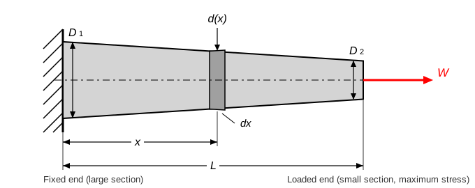
Take a slice of thickness at distance from the fixed end. The slice is short enough that the internal force and area are constant across it, so the uniform-bar result applies to the slice alone:

The total extension is the sum of all the slice extensions:

Every result in this section, and every taper, step, or self-weight problem you will meet, comes from this one integral. The uniform bar is just the special case where and come out of the integral: .

Case A: Circular Bar Tapering Linearly (the standard case)

A bar of circular section tapers uniformly from diameter at the fixed end to at the loaded end over a length , carrying an axial load .

1. Geometry. The diameter falls off linearly with :

   so the area at any section is .

2. Internal force. The bar is loaded only at its end, so at every section.

3. Substitute into the general rule:

4. Do the integral. Since :

5. Back-substitute and combine the fractions, :

   The taper difference cancels, leaving the standard result:

What the Tapered-Bar Result Tells You

• Extension: , symmetric in and , so which end is fixed makes no difference to the total extension.
• Maximum stress is at the small end, where the area is least:
• Stress at any section uses the local diameter: . At mid-length the diameter is the arithmetic mean, , giving .
• Equivalent uniform bar: setting gives , the geometric mean of the end diameters. A uniform bar of that diameter stretches exactly as much as the taper.
• Cost of tapering: compared with a uniform bar of the large diameter, the taper stretches times as much. Halving the end diameter doubles the extension.

Case B: Flat Bar of Constant Thickness and Tapering Width

A plate of constant thickness tapers linearly in width from to over length under axial load . Now , and the area appears to the first power, so the integral is a logarithm rather than a reciprocal:

The equivalent uniform width is the logarithmic mean, . Maximum stress is again at the narrow end, .

Case C: Stepped Bar (a Discrete Version of the Same Idea)

If the section changes in steps rather than continuously, the integral becomes a sum, because each segment is internally uniform:

Each segment is analysed on its own and the extensions are added. The stress is checked segment by segment, and the critical segment is the one with the largest , which is not necessarily the longest or the most heavily loaded one. Compound bars apply this same summation to segments of different materials.

Case D: When the Internal Force Varies (Self-Weight)

Self-weight problems use the identical integral, except that varies and may not:

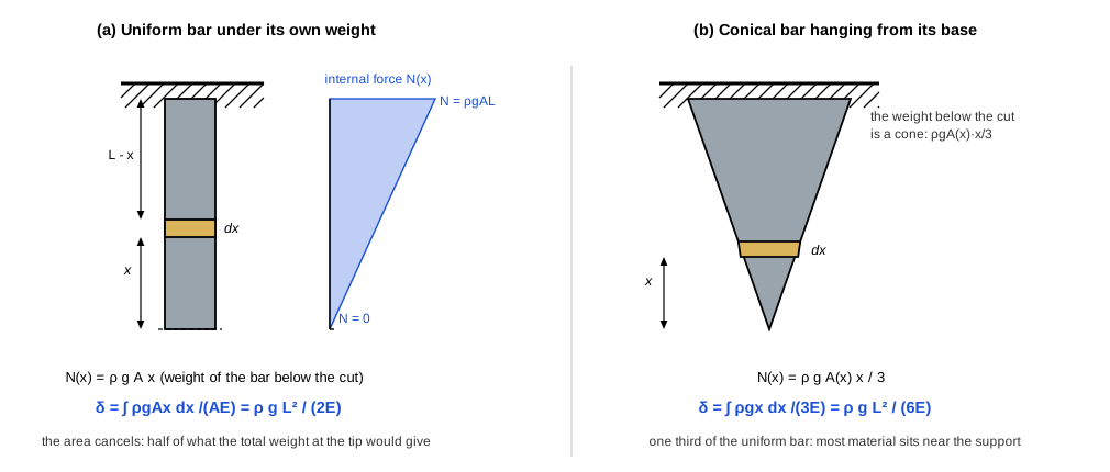
• Uniform bar hanging under its own weight ( = density, = 9.81 m/s²). At a height above the free end the bar carries the weight below it, , so

  which is exactly half the extension the total weight would produce if it were hung at the free end.

• Conical bar suspended from its base. At a distance from the apex the weight below is that of a cone, , so the area cancels again and

  one third of the uniform-bar value, because most of the material sits near the support where it carries little of the weight below it.

Summary of Varying-Section Results

Member	or	Extension	Maximum stress
Uniform bar, end load	constant
Circular taper
Flat taper , thickness	linear in
Stepped bar	piecewise constant
Uniform bar, self-weight			(at the support)
Conical bar, self-weight			(at the base)

Equivalent uniform section: for a circular taper, for a flat taper.

The Stress-Strain Curve

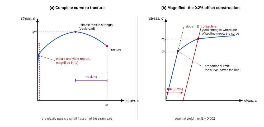
A tensile test pulls a standard coupon to fracture while recording force and extension. The resulting curve divides material behaviour into regions:

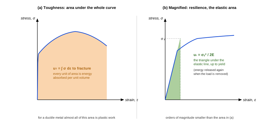
The two panels are the same curve at different scales, and the scale change is the point: the elastic behaviour that governs every deflection calculation in this lesson occupies a small fraction of the strain axis, so the 0.2% offset construction can only be drawn in the magnified view. The axes are deliberately unnumbered because the shape is common to ductile metals while the values are not; the figures for one particular steel are worked out in Application 3 below.

Key Points on the Curve

• Proportional limit: the highest stress at which stress and strain remain strictly proportional (the curve is still a straight line)
• Yield strength (0.2% offset): found by drawing a line with slope starting at ; where it intersects the curve is the yield point
• Ultimate tensile strength (UTS): the peak stress the material ever carries
• Fracture point: where the coupon breaks; the strain here gives the percent elongation (a ductility measure)

Modulus of Resilience and Modulus of Toughness

Energy Absorption Measures

Resilience measures how much elastic energy the material stores per unit volume before yielding. Toughness measures the total energy per unit volume absorbed before fracture, including all the plastic work.

Both quantities are areas under the same curve, which is why they are so easily confused, and the figure shows how different those areas are. For a ductile metal the elastic triangle is smaller than the total area by orders of magnitude, so the toughness is essentially all plastic work. Steps 2 and 3 of Application 3 evaluate both areas for a particular steel.

Shear Modulus

Shear Modulus and Its Relation to E and Poisson's Ratio

Where:

• = shear modulus (Pa or MPa)
• = shear stress (Pa or MPa)
• = shear strain (dimensionless, in radians)
• = thickness of the sheared layer

For metals, falls between and . For elastomers with , , much smaller than for metals.

Application 1: CNC Actuator Shaft, Steel vs Aluminum

The CNC Z-axis shaft must transmit a maximum axial force of 5,000 N while keeping elongation within 0.05 mm over its 400 mm length. Both a strength check and a stiffness check are required.

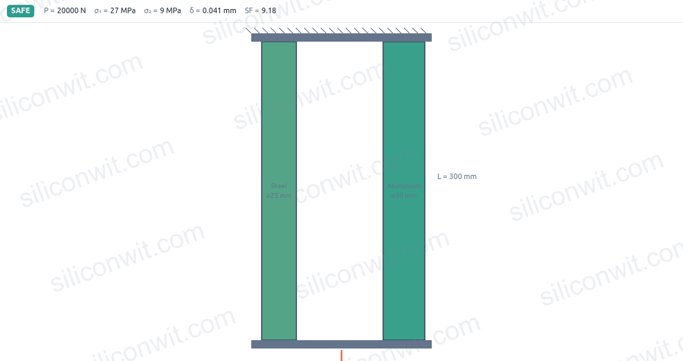
Run the steel and the aluminum shaft as the A and B states in the simulator and compare the deflection directly:

Step 1: Minimum Diameter from the Strength Criterion

Click to reveal the strength calculations

1. Allowable stress for each material with SF = 3:

   Aluminum: ✅

   Steel: ✅

2. Minimum area from :

   Aluminum: ✅

   Steel: ✅

3. Minimum diameter from :

   Aluminum: ✅

   Steel: ✅

   Strength alone would permit quite a thin shaft for either material. ✅

Step 2: Minimum Diameter from the Stiffness Criterion

Click to reveal the stiffness calculations

1. Required area from mm, rearranged to :

   Aluminum: ✅

   Steel: ✅

   (Here is in MPa = N/mm², so in mm and in mm are consistent.)

2. Required diameter from :

   Aluminum: ✅

   Steel: ✅

3. Compare the two criteria:

   For aluminum: strength needs 8.4 mm, stiffness needs 27.0 mm. Stiffness governs by a factor of 3.2. ✅

   For steel: strength needs 6.0 mm, stiffness needs 16.0 mm. Stiffness governs by a factor of 2.7. ✅

Step 3: Verify the Final Design and Compare Materials

Click to reveal the design comparison

1. Confirm deformation for the stiffness-governed diameters. For the 27 mm aluminum shaft:

   ✅

   (just within 0.05 mm) ✅

   For the 16 mm steel shaft:

   ✅

   (just within 0.05 mm) ✅

2. Estimate shaft mass using :

   Aluminum ( kg/m³): kg ✅

   Steel ( kg/m³): kg ✅

   The masses are nearly equal because steel’s higher density is almost exactly offset by its smaller cross-section. ✅

3. Design decision: Steel 1045 at 16 mm diameter meets both criteria, uses a 41% smaller diameter (16 mm versus 27 mm, which fits tighter machine envelopes), and has a similar mass to the aluminum option. ✅

Application 2: Tapered Steel Pull-Rod on the Machine Spindle

The shaft in Application 1 was uniform because it runs in bearings along its whole length. A drawbar or pull-rod is different: it is loaded in tension at one end and anchored at the other, nothing slides on it, and it moves with the axis, so every kilogram of it costs acceleration. That is exactly the case for a taper: put the metal where the stress is, and remove it where the stress is low.

Step 1: Maximum Stress and Where It Acts

Click to reveal the maximum stress calculation

1. Locate the critical section. The internal force is kN at every section (the rod is loaded only at its ends), so the stress is largest where the area is smallest, which is the loaded end at mm. No integration is involved. ✅

2. Area of the small end:

   ✅

3. Maximum stress:

   ✅

4. Compare with the large end for context:

   The stress at the small end is four times the stress at the large end, because doubling the diameter quadruples the area. The factor of safety against yield is , so this rod is stiffness-critical rather than strength-critical, exactly like the shaft in Application 1. ✅

Step 2: Total Extension of the Tapered Rod

Click to reveal the extension calculation

1. Select the relation. The area varies, so does not apply. From the derivation in the theory section, a linear circular taper gives:

2. Substitute, keeping every length in mm and in MPa = N/mm² so the answer comes out in mm:

   ✅

3. Sanity-check the magnitude. The rod is nowhere thinner than 25 mm, so its extension must lie between that of a uniform 50 mm rod and a uniform 25 mm rod:

   • Uniform 50 mm: mm
   • Uniform 25 mm: mm

   The taper result, 0.1146 mm, sits between the two, and is exactly times the uniform 50 mm value, as the formula predicts. ✅

4. What the wrong method would have given. Using the mid-length area mm²:

   That is 11.1% below the correct value. The averaging must be done on , not on . ❌

Step 3: Stress at Mid-Length

Click to reveal the mid-length stress

1. Diameter at mid-length. The diameter varies linearly, so at it is the arithmetic mean of the end diameters:

   ✅

2. Area and stress there:

   ✅

3. Note the asymmetry. The mid-length stress (22.64 MPa) is not the average of the end stresses ( MPa). Stress varies as , not linearly, so it stays low over most of the rod and rises sharply only near the small end. This is why the taper is efficient: the highly stressed material is a small fraction of the rod. ✅

4. Local strain, for reference. gives at the small end and at the large end. Strain varies along the rod, which is precisely why the extension needed an integral. ✅

Step 4: Equivalent Uniform Rod and the Mass Saved

Click to reveal the equivalence and mass comparison

1. Equivalent uniform diameter. Set the uniform-bar extension equal to the taper extension:

   ✅

   Check: mm², and mm, matching Step 2 exactly. ✅

2. Volume of the tapered rod (a frustum of a cone):

   ✅

   Mass at kg/m³: kg ✅

3. Compare with the uniform 50 mm rod (the one you would use if the anchor end sets the diameter):

   The taper saves 41.7% of the material and 5.8 kg of moving mass, at the price of doubling the extension from 0.057 mm to 0.115 mm. ✅

4. Design decision. If the deflection budget for this rod is 0.15 mm, the taper passes (0.115 mm) with a strength factor of safety above 10, and is the better design because the mass is on a moving axis. If the budget were 0.10 mm, the taper would fail on stiffness and the small end would have to be increased: from , holding mm, mm, so a 30 mm small end. ✅

Variation: The Same Method on a Flat Tapered Tie Plate

Click to reveal the flat-taper worked example

An aluminum tie plate ( GPa) of constant thickness mm tapers in width from mm at the anchor to mm at the pin, over mm, carrying kN.

1. Maximum stress at the narrow end (smallest area, mm²):

   ✅

   (At the wide end, mm² and MPa: half, because here the area is linear in the width, not quadratic.)

2. Extension from the flat-taper result:

   ✅

3. Equivalent uniform width (the logarithmic mean):

   Check: mm ✅

   Note that the equivalent width (86.6 mm) is below the arithmetic mean (90 mm), the same bias seen in the circular taper. ✅

Practice: Four Variations to Work Yourself

Click to reveal the practice problems and their answers

Work each one from the four-step recipe, then check against the answers.

1. Circular taper. A steel bar ( GPa) tapers from mm to mm over mm under kN. Find the maximum stress, the total extension, and the stress at mid-length.

   Answers: MPa at the small end; mm; mm so MPa. ✅

2. Flat taper. An aluminum plate ( GPa), thickness 8 mm, tapers from 100 mm to 50 mm wide over 500 mm under 30 kN. Find the maximum stress and the extension.

   Answers: MPa; mm. ✅

3. Design (inverse) problem. A steel taper ( GPa) has mm, mm, and carries kN. The extension must not exceed 0.15 mm. What is the smallest permissible , and what is the resulting maximum stress?

   Answers: rearranging, mm, so use 20 mm. Then mm ✅ and MPa, a factor of safety of 4.8 against a 530 MPa yield. ✅

4. Self-weight. A uniform steel bar hangs vertically from its top end, m, kg/m³, GPa, carrying no other load. Find the extension and the maximum stress.

   Answers: m mm; MPa at the top support, where the whole weight is carried. Note the area never entered either answer. ✅

Application 3: Interpreting a Tensile Test of a Steel Coupon

A tensile test is the standard way to measure the mechanical properties of a material before it goes into a design. Understanding how to read the stress-strain curve lets you extract the numbers that feed every other analysis.

Step 1: Confirm the 0.2% Offset Yield Construction

Click to reveal the 0.2% offset construction

1. What “0.2% offset” means. Draw a straight line with slope equal to (200 GPa) that starts not at the origin but at on the strain axis. Where that line intersects the actual stress-strain curve is defined as the yield strength. The 0.002 offset accounts for the permanent set that is considered acceptable for a yield criterion.

2. Check the elastic slope at the yield point. At MPa the elastic strain is:

   ✅

   The total strain at the 0.2% offset yield point is , which is consistent with where the offset line meets the curve. ✅

3. Read the other landmarks:

   • Proportional limit MPa at strain (curve is still linear)
   • UTS = 520 MPa at a strain of roughly 12% (the peak of the curve)
   • Fracture at 22% elongation and 410 MPa (necking has reduced the load-bearing area)

Step 2: Modulus of Resilience

Click to reveal the resilience calculation

1. Formula. The modulus of resilience is the area under the elastic portion of the curve, approximated as a triangle:

2. Calculation:

   ✅

3. Meaning. This steel can absorb 306 kJ per cubic metre elastically before yielding. A material with higher resilience makes a better spring; higher toughness (see Step 3) makes a better crash absorber. ✅

Step 3: Estimate the Modulus of Toughness

Click to reveal the toughness estimate

1. Approach. The modulus of toughness is the total area under the stress-strain curve. A practical estimate splits the curve into the elastic triangle plus a trapezoidal plastic region:

   where is the strain at yield (approximately 0.00175) and .

2. Calculation:

   Elastic contribution: J/m³ (from Step 2) ✅

   Average stress over plastic region: MPa ✅

   Plastic strain range: ✅

   Plastic contribution: J/m³ MJ/m³ ✅

   Total: MJ/m³ ✅

3. Interpretation. The steel absorbs roughly 95 MJ per cubic metre before fracturing. Nearly all of that (99.7%) is plastic work during the large permanent elongation. This high toughness is what makes medium-carbon steel suitable for parts that must absorb impact without shattering. ✅

Step 4: Percent Elongation (Ductility)

Click to reveal the percent elongation

1. Percent elongation is defined over the original gauge length:

   ✅

   (The fracture elongation of 22% was read from the curve; it means the gauge section grew from 50 mm to 61 mm before breaking.) ✅

2. Classification. Materials with are considered ductile. At 22%, this steel has substantial ductility: it gives visual warning (necking and elongation) well before fracture, which is the property that makes ductile metals forgiving in overload situations. ✅

Application 4: Shear Modulus and a Bonded Elastomer Anti-Vibration Mount

Shear modulus governs any component that is loaded across its thickness rather than along its length. Bonded elastomer mounts are a common example: the rubber layer is glued between two metal plates, and when the structure moves horizontally the rubber is sheared. The mount’s compliance in shear is exactly what provides the vibration isolation.

Step 1: Shear Modulus from E and Poisson’s Ratio

Click to reveal the shear modulus calculation

1. Apply the elastic relation between , , and :

   ✅

2. Context. For nearly incompressible materials such as rubber ( to ), the denominator approaches , so . This is why rubber is much easier to shear than to compress: its shear modulus is only a third of its tensile modulus, while for steel the ratio is about . ✅

Step 2: Shear Stress in the Rubber Layer

Click to reveal the shear stress calculation

1. Shear stress is force over the area parallel to the load:

   ✅

2. Check against the rubber’s short-term shear strength. Natural rubber typically carries shear stresses up to 1 to 2 MPa before tearing. At 0.125 MPa the mount is well within its elastic range. ✅

Step 3: Shear Strain and Lateral Deflection

Click to reveal the shear strain and deflection

1. Shear strain from :

   ✅

2. Lateral shear deflection. Shear strain is the tangent of the shear angle, which for small angles equals :

   ✅

3. Interpret the result. A lateral deflection of about 1.9 mm under 800 N gives a lateral stiffness of N/mm. Anti-vibration mounts for light machinery typically target lateral stiffnesses in the range of 200 to 800 N/mm, so this mount is in the right design region. ✅

Design Guidelines for Strain and Material Properties

Summary and Next Steps

Key Concepts Mastered

1. Axial deflection follows . In precision systems the stiffness criterion (deformation limit) almost always sets a larger minimum section than the strength criterion, and both must be checked.
2. Non-uniform members are all handled by one relation, : a linear circular taper gives , a flat taper gives , a stepped bar gives , and self-weight gives for a uniform bar. The maximum stress is always at the smallest section and needs no integration; the extension can never be found from an average area.
3. The tensile test curve captures stiffness (, the slope), yield strength (0.2% offset construction), UTS (peak), fracture strain (ductility), and the energy per unit volume the material can absorb (resilience and toughness).
4. Shear modulus is related to Young’s modulus and Poisson’s ratio by . Shear-loaded parts (elastomer mounts, pins, adhesive joints) use and to find the shear deflection .

Results at a Glance

Application	Key result	Governing criterion
CNC shaft: aluminum 27 mm, steel 16 mm	Al: mm, mass 0.62 kg; steel: mm, mass 0.63 kg	Stiffness governs both
Tapered pull-rod (50 mm → 25 mm, 900 mm, 25 kN)	MPa at the small end, mm, MPa, mm, 41.7% less material	Stiffness governs (SF = 10.4 on strength)
Steel tensile coupon	kJ/m³, MJ/m³, ductility 22%	Yield at 350 MPa, UTS 520 MPa
Elastomer mount (80 mm x 80 mm, 20 mm thick)	MPa, MPa, rad, mm	Shear governs deflection

A Note on Tools

Every number in this lesson came from four relations (, its non-uniform form , , and ) and a calculator. Finite-element software is not needed for axial or shear members, tapered ones included; the hand calculation is the design, and simulation is for validating complex geometry after the sizing is done.

Next, Compound Bars and Composite Systems extends the axial analysis to members made of two different materials in series or parallel, which is the situation in every bolted joint, press fit, and bi-material actuator.

Comments

Loading comments...