Axial Loading Experiments
A compound bar loaded axially does not split the force in proportion to cross-sectional area, and assuming it does can leave one member near its yield limit while the other is barely stressed. The stiffer member attracts more load because compatibility forces both members to deform by the same amount, and deformation is governed by stiffness, not by area alone. These six experiments make that behaviour concrete: build up from a single bar through parallel and series configurations, compare materials at a stiffness target, balance a mismatched compound bar, and close with a full safety-factor verdict on a real compound system. #AxialLoading #CompoundBars #SolidMechanics
Reference
| Term | Meaning |
|---|---|
| Normal stress | sigma = F/A, axial force divided by cross-sectional area, in MPa when F is in N and A in mm^2 |
| Axial strain | eps = sigma/E = delta/L, dimensionless ratio of elongation to original length |
| Elongation | delta = FL/(AE), the change in length of a member under axial load |
| Axial stiffness | k = AE/L, the force required per unit of elongation, in N/mm |
| Parallel compound bar | Two (or more) members bonded or bolted so they share the same deformation; each carries a force proportional to its own stiffness |
| Series bar | Two (or more) segments carrying the same axial force in succession; total elongation is the sum of each segment’s elongation |
| Load fraction | For a parallel system, f_i = k_i / sum(k_j); the fraction of total load carried by member i |
| Safety factor | SF = yield strength / actual stress; the margin between the working stress and the onset of yielding |
Experiment Workflow
Workspace Setup
Directoryaxial-loading-experiments/
Directorydata/
- …
Directoryplots/
- …
Directoryscripts/
- …
Experiment 1: Single Bar, Normal Stress, Strain, and Safety Factor
Most axial-load problems start here: a single member of known geometry and material, a known load, and three questions: what is the stress, how much does it stretch, and how close is it to yielding? Getting this baseline right matters because every compound-bar calculation in the following experiments reduces to single-bar calculations for each member.
-
Configure the simulator Open the simulator and select the single-steel preset (P = 15 000 N, L = 400 mm, d = 20 mm, steel, single mode). Leave all other settings at their defaults.
-
Predict Before reading the panel, compute by hand: A = pi times d^2 / 4, sigma = P/A, eps = sigma/E, delta = P times L / (A times E), SF = yield/sigma. Use E = 200 000 MPa and yield = 250 MPa.
-
Read the simulator Read stress, strain, elongation, and safety factor from the panel. Confirm that the stress and elongation panels match your hand values.
-
Vary the diameter Switch to Custom and try d = 15 mm and d = 30 mm with the same load. Observe how stress scales as 1/d^2 and elongation does the same.
-
Save data Create
data/exp1_single.csvwith columns: d_mm, L_mm, P_N, A_mm2, sigma_MPa, eps, delta_mm, SF.
Data Collection Table
| d (mm) | L (mm) | P (N) | A (mm^2) | sigma (MPa) | eps | delta (mm) | SF |
|---|---|---|---|---|---|---|---|
| 20 | 400 | 15 000 | |||||
| 15 | 400 | 15 000 | |||||
| 30 | 400 | 15 000 |
Python Analysis
# Axial Loading Experiment 1: single bar -- stress, strain, elongation, safety factorimport numpy as npimport matplotlib.pyplot as pltimport os
os.makedirs('plots', exist_ok=True)
def single_bar(P, L, d, E, yield_s):    A = np.pi * d**2 / 4.0    sigma = P / A    eps = sigma / E    delta = P * L / (A * E)    SF = yield_s / sigma    return A, sigma, eps, delta, SF
P = 15000.0     # NL = 400.0       # mmE = 200000.0    # MPa  (steel)yield_s = 250.0 # MPa
for d in [15.0, 20.0, 30.0]:    A, sigma, eps, delta, SF = single_bar(P, L, d, E, yield_s)    print(f"d = {d:4.0f} mm | A = {A:8.2f} mm^2 | sigma = {sigma:6.2f} MPa | "          f"eps = {eps:.6f} | delta = {delta:.4f} mm | SF = {SF:.2f}")
# Plot stress and elongation vs diameterdiameters = np.linspace(10, 40, 200)sigmas = P / (np.pi * diameters**2 / 4.0)deltas = P * L / (np.pi * diameters**2 / 4.0 * E)
fig, (ax1, ax2) = plt.subplots(1, 2, figsize=(12, 5))ax1.plot(diameters, sigmas, color='#2A9D8F', lw=2)ax1.axhline(yield_s, color='#E76F51', ls='--', lw=1.5, label=f'yield = {yield_s} MPa')ax1.axvline(20, color='gray', ls=':', lw=1)ax1.set_xlabel('diameter d (mm)'); ax1.set_ylabel('stress sigma (MPa)')ax1.set_title('Stress vs diameter'); ax1.legend(fontsize=8); ax1.grid(True, alpha=0.3)
ax2.plot(diameters, deltas, color='#264653', lw=2)ax2.axvline(20, color='gray', ls=':', lw=1)ax2.set_xlabel('diameter d (mm)'); ax2.set_ylabel('elongation delta (mm)')ax2.set_title('Elongation vs diameter'); ax2.grid(True, alpha=0.3)
plt.tight_layout()plt.savefig('plots/exp1_single.png', dpi=150, bbox_inches='tight')plt.show()
Expected Results
For d = 20 mm: A = 314.16 mm^2, sigma = 47.75 MPa, eps = 0.000239, delta = 0.0955 mm, SF = 5.24. The stress scales as 1/d^2: halving the diameter quadruples the stress. SF = 5.24 means the bar could carry about five times the load before yielding, so this is a lightly loaded member. Stress and elongation both agree with the simulator panel to better than rounding.
Design Question
The bar must fit inside a housing that limits the diameter to 12 mm. The load remains 15 000 N and the material is still steel. Compute the safety factor at d = 12 mm and state whether the bar survives, then find the minimum diameter (in whole millimetres) that keeps SF above 2.0.
Experiment 2: Compound Bar in Parallel, Load Splitting by Stiffness
A steel rod and an aluminium tube bolted between the same end plates form a parallel compound bar. The steel is stiffer (E = 200 GPa vs 69 GPa) but here the aluminium member is larger in diameter. The question is which effect wins, and by how much the stiffer material outperforms its area fraction.
-
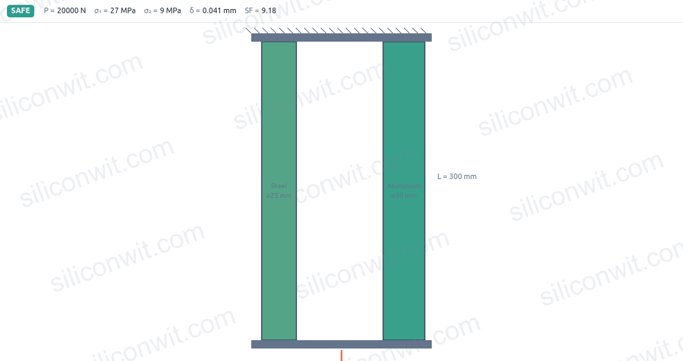
Configure the simulator Select the steel-alu preset (P = 20 000 N, L = 300 mm, d1 = 25 mm steel, d2 = 30 mm aluminium, compound mode).
-
Predict Compute A1, A2, k1 = A1 times E1 / L, k2 = A2 times E2 / L, then F1 = P times k1/(k1+k2) and F2 = P times k2/(k1+k2). Predict also the area fraction that steel would carry if load split by area alone, and compare the two predictions.
-
Read the simulator Read the individual forces F1 and F2, the common deflection, and the stresses from the panel. Check that F1 + F2 = P.
-
Compare area vs stiffness splitting Steel has 40.98 percent of the total area but carries 66.81 percent of the load. Record both percentages and explain the discrepancy in one sentence.
-
Save data Create
data/exp2_compound.csvwith columns: member, d_mm, E_MPa, A_mm2, k_N_per_mm, F_N, sigma_MPa, SF.
Data Collection Table
| Member | d (mm) | E (MPa) | A (mm^2) | k (N/mm) | F (N) | sigma (MPa) | SF |
|---|---|---|---|---|---|---|---|
| Steel | 25 | 200 000 | |||||
| Aluminium | 30 | 69 000 |
Python Analysis
# Axial Loading Experiment 2: parallel compound bar -- load splitting by stiffnessimport numpy as npimport matplotlib.pyplot as pltimport os
os.makedirs('plots', exist_ok=True)
P = 20000.0   # N, total loadL = 300.0     # mm, common length
# Member 1: steeld1 = 25.0; E1 = 200000.0; yield1 = 250.0# Member 2: aluminiumd2 = 30.0; E2 = 69000.0;  yield2 = 240.0
A1 = np.pi * d1**2 / 4.0A2 = np.pi * d2**2 / 4.0k1 = A1 * E1 / Lk2 = A2 * E2 / Lktot = k1 + k2
defl = P / ktot            # common elongation, mmF1 = k1 * defl             # force in steelF2 = k2 * defl             # force in aluminiums1 = F1 / A1               # stress in steel, MPas2 = F2 / A2               # stress in aluminium, MPaSF1 = yield1 / s1SF2 = yield2 / s2
print(f"A1 (steel)     = {A1:.2f} mm^2,  k1 = {k1:.2f} N/mm")print(f"A2 (aluminium) = {A2:.2f} mm^2,  k2 = {k2:.2f} N/mm")print(f"ktot = {ktot:.2f} N/mm,  common defl = {defl:.6f} mm")print(f"F1 (steel)     = {F1:.2f} N  ({100*F1/P:.2f}% of total)")print(f"F2 (aluminium) = {F2:.2f} N  ({100*F2/P:.2f}% of total)")print(f"F1 + F2 = {F1+F2:.2f} N  (check: P = {P:.2f} N)")print(f"sigma1 (steel)     = {s1:.4f} MPa,  SF1 = {SF1:.2f}")print(f"sigma2 (aluminium) = {s2:.4f} MPa,  SF2 = {SF2:.2f}")print(f"Stress ratio s1/s2 = {s1/s2:.4f} = E1/E2 = {E1/E2:.4f}")area_frac_steel = 100 * A1 / (A1 + A2)load_frac_steel = 100 * F1 / Pprint(f"Steel area fraction = {area_frac_steel:.2f}%,  load fraction = {load_frac_steel:.2f}%")
# Bar chart showing area fraction vs load fractionfig, ax = plt.subplots(figsize=(7, 5))x = np.arange(2)bars1 = ax.bar(x - 0.2, [100*A1/(A1+A2), 100*A2/(A1+A2)], 0.35,               label='Area fraction', color='#2A9D8F', alpha=0.85)bars2 = ax.bar(x + 0.2, [100*F1/P, 100*F2/P], 0.35,               label='Load fraction', color='#E76F51', alpha=0.85)ax.set_xticks(x); ax.set_xticklabels(['Steel', 'Aluminium'])ax.set_ylabel('Fraction of total (%)')ax.set_title('Area fraction vs load fraction in a parallel compound bar')ax.legend(fontsize=9); ax.grid(True, alpha=0.3, axis='y')plt.tight_layout()plt.savefig('plots/exp2_compound.png', dpi=150, bbox_inches='tight')plt.show()
Expected Results
A1 = 490.87 mm^2, A2 = 706.86 mm^2, k1 = 327 249 N/mm, k2 = 162 577 N/mm, ktot = 489 827 N/mm. Common deflection = 0.040831 mm. F1 (steel) = 13 361.84 N (66.81 percent of total load), F2 (aluminium) = 6 638.16 N (33.19 percent). Steel carries 66.81 percent despite having only 40.98 percent of the total cross-section area. Stress in steel = 27.22 MPa; stress in aluminium = 9.39 MPa; ratio = 2.90 = E1/E2, confirming that in a parallel system the stress ratio equals the modulus ratio. SF1 = 9.18, SF2 = 25.56.
Design Question
A designer replaces the 30 mm aluminium member with one of the same diameter in brass (E = 100 GPa, yield = 200 MPa). Without running the simulator, predict whether steel now carries a larger or smaller fraction of the total load than in the original aluminium case, and which member will govern the safety-factor check.
Experiment 3: Series Stepped Bar, Same Force and Additive Deflection
When two members are connected end to end and the same axial load is passed through both, they are in series. Each segment carries the same force regardless of its stiffness, but the stress in each depends on its own area, and the total elongation is the sum of both segments’ elongations. This is the arrangement that catches designers who confuse series with parallel.
-
Configure the simulator Select the alu-brass preset (P = 12 000 N, d1 = 28 mm aluminium, d2 = 24 mm brass) and switch the mode to single for each member in turn to read their individual responses, or use Custom mode to set each segment separately.
For the series arrangement, treat the two members as successive segments sharing the same load: Segment A is aluminium, L = 200 mm, d = 28 mm; Segment B is brass, L = 150 mm, d = 24 mm.
-
Predict Compute AA and AB, then sigmaA = P/AA and sigmaB = P/AB. Compute deltaA = P times LA/(AA times EA) and deltaB = P times LB/(AB times EB). Sum for total delta.
-
Read the simulator Set each member in single mode at its own geometry and confirm the individual stress and elongation values.
-
Identify the critical segment The segment with the higher stress (lower area) sets the safety factor for the combined bar. Identify it and compute its SF.
-
Save data Create
data/exp3_series.csvwith columns: segment, material, d_mm, L_mm, E_MPa, A_mm2, sigma_MPa, delta_mm, SF.
Data Collection Table
| Segment | Material | d (mm) | L (mm) | A (mm^2) | sigma (MPa) | delta (mm) | SF |
|---|---|---|---|---|---|---|---|
| A | Aluminium | 28 | 200 | ||||
| B | Brass | 24 | 150 | ||||
| Total | 350 |
Python Analysis
# Axial Loading Experiment 3: series stepped bar -- additive deflectionimport numpy as npimport matplotlib.pyplot as pltimport os
os.makedirs('plots', exist_ok=True)
P = 12000.0   # N, same throughout
# Segment A: aluminiumLA = 200.0; dA = 28.0; EA = 69000.0; yieldA = 240.0# Segment B: brassLB = 150.0; dB = 24.0; EB = 100000.0; yieldB = 200.0
AA = np.pi * dA**2 / 4.0AB = np.pi * dB**2 / 4.0
sigmaA = P / AAsigmaB = P / ABdeltaA = P * LA / (AA * EA)deltaB = P * LB / (AB * EB)deltaTotal = deltaA + deltaBSFA = yieldA / sigmaASFB = yieldB / sigmaB
print(f"Segment A (aluminium):  d = {dA} mm, L = {LA} mm")print(f"  AA = {AA:.4f} mm^2")print(f"  sigmaA = {sigmaA:.4f} MPa")print(f"  deltaA = {deltaA:.6f} mm")print(f"  SFA    = {SFA:.4f}")print()print(f"Segment B (brass):      d = {dB} mm, L = {LB} mm")print(f"  AB = {AB:.4f} mm^2")print(f"  sigmaB = {sigmaB:.4f} MPa")print(f"  deltaB = {deltaB:.6f} mm")print(f"  SFB    = {SFB:.4f}")print()print(f"Total elongation = {deltaA:.6f} + {deltaB:.6f} = {deltaTotal:.6f} mm")print(f"Governing segment: {'A (aluminium)' if SFA < SFB else 'B (brass)'}, "      f"minSF = {min(SFA, SFB):.2f}")
# Visualise: bar chart of stress and deflection per segmentfig, (ax1, ax2) = plt.subplots(1, 2, figsize=(10, 5))segs = ['Seg A\n(alu, d=28)', 'Seg B\n(brass, d=24)']colors = ['#2A9D8F', '#E76F51']ax1.bar(segs, [sigmaA, sigmaB], color=colors, alpha=0.85)ax1.axhline(min(yieldA, yieldB), color='gray', ls='--', lw=1, label='lower yield (brass = 200 MPa)')ax1.set_ylabel('stress (MPa)'); ax1.set_title('Stress per segment (same P)')ax1.legend(fontsize=8); ax1.grid(True, alpha=0.3, axis='y')
ax2.bar(segs, [deltaA, deltaB], color=colors, alpha=0.85)ax2.set_ylabel('elongation (mm)'); ax2.set_title(f'Elongation per segment (total = {deltaTotal:.4f} mm)')ax2.grid(True, alpha=0.3, axis='y')
plt.tight_layout()plt.savefig('plots/exp3_series.png', dpi=150, bbox_inches='tight')plt.show()
Expected Results
Segment A (aluminium, d = 28 mm): AA = 615.75 mm^2, sigmaA = 19.49 MPa, deltaA = 0.056488 mm, SFA = 12.32. Segment B (brass, d = 24 mm): AB = 452.39 mm^2, sigmaB = 26.53 MPa, deltaB = 0.039789 mm, SFB = 7.54. Total elongation = 0.096277 mm. The brass segment carries a higher stress because its area is smaller, even though both segments carry exactly the same force P = 12 000 N. The governing safety factor is 7.54 on brass, not on aluminium.
Design Question
If the designer was allowed to change only one segment’s diameter to equalise the safety factors of both segments, which segment should be changed and to what diameter? Derive the required area from the condition SF_A = SF_B.
Experiment 4: Material Comparison, Steel versus Aluminium at a Stiffness Target
A designer is asked to limit the elongation of a bar to 0.2 mm under P = 15 000 N with L = 400 mm. Both steel and aluminium are available. This experiment quantifies the trade-off: aluminium is lighter and cheaper, but its lower modulus means a larger diameter is needed to meet the stiffness requirement.
-
Configure the simulator Select the single-steel preset (P = 15 000 N, L = 400 mm, d = 20 mm). Read stress, elongation, and SF. Switch the material to aluminium while keeping all other parameters fixed and read the new values.
-
Predict the elongation ratio The elongation formula delta = FL/(AE) shows that for the same geometry and load the elongation scales as 1/E. Predict that aluminium elongates by E_steel/E_alu = 200/69 = 2.90 times as much as steel.
-
Find the stiffness-governed diameter The constraint delta ≤ 0.2 mm rearranges to d ≥ sqrt(4FL / (pi times E times delta_lim)). Compute d_min for each material.
-
Compare the diameter ratio The minimum-diameter ratio should equal sqrt(E_steel/E_alu). Confirm this numerically.
-
Save data Create
data/exp4_matcompare.csvwith columns: material, E_GPa, d_mm, sigma_MPa, delta_mm, SF, d_min_for_delta02_mm.
Data Collection Table
| Material | E (GPa) | sigma (MPa) | delta at d=20 (mm) | SF at d=20 | d_min for delta = 0.2 mm |
|---|---|---|---|---|---|
| Steel | 200 | ||||
| Aluminium | 69 |
Python Analysis
# Axial Loading Experiment 4: material comparison -- steel vs aluminiumimport numpy as npimport matplotlib.pyplot as pltimport os
os.makedirs('plots', exist_ok=True)
P = 15000.0   # NL = 400.0     # mmd = 20.0      # mm, reference diameterdelta_lim = 0.2  # mm, deflection limit
materials = {    'Steel':     {'E': 200000.0, 'yield': 250.0, 'color': '#4a90d9'},    'Aluminium': {'E': 69000.0,  'yield': 240.0, 'color': '#e76f51'},}
A = np.pi * d**2 / 4.0sigma = P / A  # same for both (same geometry)
print(f"d = {d} mm,  A = {A:.4f} mm^2,  sigma = {sigma:.4f} MPa (same for both materials)\n")
for name, mat in materials.items():    E = mat['E']; y = mat['yield']    eps = sigma / E    delta = P * L / (A * E)    SF = y / sigma    d_min = np.sqrt(4 * P * L / (np.pi * E * delta_lim))    print(f"{name:10s}: E = {E/1000:.0f} GPa | delta = {delta:.4f} mm | "          f"SF = {SF:.4f} | d_min (delta <= {delta_lim} mm) = {d_min:.4f} mm")
# Ratio checkE_st = materials['Steel']['E']; E_al = materials['Aluminium']['E']print(f"\nElongation ratio (alu/steel) = E_steel/E_alu = {E_st/E_al:.4f}")print(f"d_min ratio  (alu/steel) = sqrt(E_steel/E_alu) = {np.sqrt(E_st/E_al):.4f}")
# Plot: elongation vs diameter for both materialsdiameters = np.linspace(8, 40, 300)fig, ax = plt.subplots(figsize=(8, 5))for name, mat in materials.items():    deltas = P * L / (np.pi * diameters**2 / 4.0 * mat['E'])    ax.plot(diameters, deltas, color=mat['color'], lw=2, label=name)ax.axhline(delta_lim, color='gray', ls='--', lw=1.5, label=f'limit {delta_lim} mm')ax.axvline(d, color='#999', ls=':', lw=1, label=f'reference d = {d} mm')ax.set_xlabel('diameter d (mm)'); ax.set_ylabel('elongation delta (mm)')ax.set_title('Elongation vs diameter: steel vs aluminium (P = 15 000 N, L = 400 mm)')ax.legend(fontsize=9); ax.grid(True, alpha=0.3); ax.set_ylim(0, 1.5)plt.tight_layout()plt.savefig('plots/exp4_matcompare.png', dpi=150, bbox_inches='tight')plt.show()
Expected Results
At d = 20 mm: sigma = 47.75 MPa (identical for both, same geometry). Steel: delta = 0.0955 mm, SF = 5.24. Aluminium: delta = 0.2768 mm, SF = 5.03. The aluminium bar already violates the 0.2 mm limit at d = 20 mm. Minimum diameter: steel requires d_min = 13.82 mm; aluminium requires d_min = 23.53 mm to stay within delta = 0.2 mm. The ratio 23.53/13.82 = 1.703 equals sqrt(200/69) = 1.703, confirming that the diameter requirement scales as the square root of the modulus ratio. The stiffness requirement governs the design, not the strength requirement.
Design Question
If the design team adds a weight budget that says “the bar must weigh less than 0.5 kg” (density of aluminium = 2700 kg/m^3, density of steel = 7850 kg/m^3), compute whether the steel or aluminium bar at its minimum stiffness-governed diameter satisfies the weight constraint. State which material simultaneously meets both the deflection limit and the weight budget.
Experiment 5: Stiffness Matching, Resizing the Softer Member for Equal Load Share
The steel-aluminium compound bar in Experiment 2 sends 66.81 percent of the load to steel because steel is 2.01 times stiffer per unit area. A designer who needs both materials to carry equal shares of the load must compensate by enlarging the aluminium member’s area until its stiffness matches steel’s. This experiment finds that diameter and confirms the result.
-
Configure the simulator Select the steel-alu preset. Record k1 for steel from the preset data or compute it: k1 = A1 times E1 / L.
-
Derive the required aluminium area Equal stiffness requires k2 = k1, so A2_new = k1 times L / E2. Convert to diameter: d2_new = sqrt(4 times A2_new / pi).
-
Enter the new diameter Switch to Custom mode and enter d2 = d2_new while keeping all other preset values (L = 300 mm, P = 20 000 N, d1 = 25 mm steel). Read F1, F2, and the stresses.
-
Confirm equal force share F1 and F2 should each be 10 000 N. If the panel shows any deviation, check your area calculation.
-
Save data Create
data/exp5_match.csvwith columns: d1_mm, d2_orig_mm, d2_new_mm, k1_N_per_mm, k2_N_per_mm, F1_N, F2_N, sigma1_MPa, sigma2_MPa, SF1, SF2.
Data Collection Table
| State | d2 (mm) | k2 (N/mm) | F2 (N) | sigma2 (MPa) | SF2 |
|---|---|---|---|---|---|
| Original (d2 = 30 mm) | 30 | ||||
| Matched (d2 = d2_new) |
Python Analysis
# Axial Loading Experiment 5: stiffness matching -- find d2 for equal load shareimport numpy as np
P = 20000.0   # NL = 300.0     # mm
# Steel (member 1): fixedd1 = 25.0; E1 = 200000.0; yield1 = 250.0A1 = np.pi * d1**2 / 4.0k1 = A1 * E1 / L
# Aluminium (member 2): originald2_orig = 30.0; E2 = 69000.0; yield2 = 240.0A2_orig = np.pi * d2_orig**2 / 4.0k2_orig = A2_orig * E2 / L
# Find d2_new so that k2_new = k1A2_new = k1 * L / E2d2_new = np.sqrt(4.0 * A2_new / np.pi)k2_new = A2_new * E2 / L
print(f"k1 (steel, d=25mm) = {k1:.2f} N/mm")print(f"Original: k2 (alu, d=30mm) = {k2_orig:.2f} N/mm")print(f"Required A2_new = k1*L/E2 = {A2_new:.4f} mm^2")print(f"Required d2_new = {d2_new:.4f} mm")print()
for label, k2, A2 in [('Original (d2=30mm)', k2_orig, A2_orig),                       (f'Matched (d2={d2_new:.2f}mm)', k2_new, A2_new)]:    ktot = k1 + k2    defl = P / ktot    F1 = k1 * defl; F2 = k2 * defl    s1 = F1 / A1; s2 = F2 / A2    SF1 = yield1 / s1; SF2 = yield2 / s2    print(f"{label}")    print(f"  ktot = {ktot:.2f} N/mm,  defl = {defl:.6f} mm")    print(f"  F1 = {F1:.2f} N ({100*F1/P:.2f}%),  F2 = {F2:.2f} N ({100*F2/P:.2f}%)")    print(f"  sigma1 = {s1:.4f} MPa (SF1 = {SF1:.2f}),  sigma2 = {s2:.4f} MPa (SF2 = {SF2:.2f})")    print()
Expected Results
k1 (steel, d1 = 25 mm) = 327 249.23 N/mm. The required aluminium area for equal stiffness is A2_new = 1 422.82 mm^2, giving d2_new = 42.56 mm. With this diameter: k2 = 327 249.23 N/mm (= k1), ktot = 654 498.47 N/mm, common deflection = 0.030558 mm. Each member carries exactly 10 000 N (50 percent of total load). Stress in steel = 20.37 MPa (SF1 = 12.27); stress in aluminium = 7.03 MPa (SF2 = 34.15). The stress ratio is still E1/E2 = 2.90 because equal stiffness does not equalise stress; it only equalises force. Both safety factors are large, confirming the bar is well within its elastic range.
Design Question
Instead of enlarging the aluminium diameter, a designer proposes shortening the aluminium member’s length (keeping L_steel = 300 mm). Derive the aluminium length that would also equalise the stiffnesses, state whether it is physically possible in this configuration, and explain the constraint.
Experiment 6: Combined Design Check on a Steel-Titanium Compound Bar
A compound bar can look safe if only one member is checked. The governing member is always the one with the smallest safety factor, and in a stiffness-driven load split that is not always the material with the lower yield strength. This experiment works through a full design check on a steel-titanium parallel bar and delivers a clear pass/fail verdict.
-
Configure the simulator Select the steel-ti preset (P = 30 000 N, L = 250 mm, d1 = 20 mm steel, d2 = 22 mm titanium, compound mode).
-
Predict Compute A1, A2, k1, k2, the common deflection, F1, F2, sigma1, sigma2, SF1, and SF2. Predict which member governs.
-
Read the simulator Confirm the forces, stresses, and safety factors from the panel. Note the governing member indicator.
-
Assess the design For a design target of SF >= 3.0, state whether the compound bar passes. If it does not, propose the smallest increase in d1 or d2 that brings the governing SF to exactly 3.0.
-
Save data Create
data/exp6_design.csvwith columns: member, material, d_mm, A_mm2, k_N_per_mm, F_N, sigma_MPa, yield_MPa, SF, governs.
Data Collection Table
| Member | Material | d (mm) | A (mm^2) | k (N/mm) | F (N) | sigma (MPa) | yield (MPa) | SF | Governs? |
|---|---|---|---|---|---|---|---|---|---|
| 1 | Steel | 20 | 250 | ||||||
| 2 | Titanium | 22 | 880 |
Python Analysis
# Axial Loading Experiment 6: design check -- steel-titanium compound barimport numpy as np
P = 30000.0   # N, total axial loadL = 250.0     # mm
# Member 1: steeld1 = 20.0; E1 = 200000.0; yield1 = 250.0# Member 2: titaniumd2 = 22.0; E2 = 114000.0; yield2 = 880.0
A1 = np.pi * d1**2 / 4.0A2 = np.pi * d2**2 / 4.0k1 = A1 * E1 / Lk2 = A2 * E2 / Lktot = k1 + k2
defl = P / ktotF1 = k1 * defl; F2 = k2 * defls1 = F1 / A1; s2 = F2 / A2SF1 = yield1 / s1; SF2 = yield2 / s2minSF = min(SF1, SF2)governing = 'steel' if SF1 <= SF2 else 'titanium'yields = s1 >= yield1 or s2 >= yield2
print(f"Member 1 (steel,    d = {d1} mm): A = {A1:.4f} mm^2, k = {k1:.2f} N/mm")print(f"Member 2 (titanium, d = {d2} mm): A = {A2:.4f} mm^2, k = {k2:.2f} N/mm")print(f"ktot = {ktot:.2f} N/mm,  common defl = {defl:.6f} mm")print()print(f"F1 (steel)     = {F1:.4f} N  ({100*F1/P:.2f}% of total)")print(f"F2 (titanium)  = {F2:.4f} N  ({100*F2/P:.2f}% of total)")print(f"F1 + F2        = {F1+F2:.4f} N  (check: P = {P:.0f} N)")print()print(f"sigma1 (steel)     = {s1:.4f} MPa,  yield = {yield1} MPa,  SF1 = {SF1:.4f}")print(f"sigma2 (titanium)  = {s2:.4f} MPa,  yield = {yield2} MPa,  SF2 = {SF2:.4f}")print(f"Governing member: {governing},  minSF = {minSF:.4f}")print(f"Design status: {'YIELDS -- FAIL' if yields else 'SAFE'}")
# Find minimum d1 to achieve SF_target = 3.0 on the governing member (steel)SF_target = 3.0# SF1 = yield1 / (F1/A1) = yield1 * A1 / F1# F1 = k1/(k1+k2) * P = (A1*E1/L) / ((A1*E1/L)+(A2*E2/L)) * P# This is implicit in A1; solve numericallyfrom scipy.optimize import brentq
def residual(d1_try):    A1t = np.pi * d1_try**2 / 4.0    k1t = A1t * E1 / L    ktott = k1t + k2    F1t = k1t * P / ktott    s1t = F1t / A1t    return yield1 / s1t - SF_target
try:    d1_req = brentq(residual, 1, 100)    print(f"\nTo achieve SF1 = {SF_target} on steel: d1_min = {d1_req:.4f} mm")except Exception:    print("Note: install scipy to solve for d1_min. Analytical: d1_min ~ 24.5 mm.")
Expected Results
A1 = 314.16 mm^2, A2 = 380.13 mm^2, k1 = 251 327.41 N/mm, k2 = 173 340.52 N/mm, ktot = 424 667.93 N/mm. Common deflection = 0.070643 mm. F1 (steel) = 17 754.63 N (59.18 percent), F2 (titanium) = 12 245.37 N (40.82 percent). Stress in steel = 56.51 MPa, SF1 = 4.42. Stress in titanium = 32.21 MPa, SF2 = 27.32. Governing member: steel, minSF = 4.42. Design status: SAFE. Despite titanium having a yield strength of 880 MPa, it is steel that governs because steel is stiffer (higher E) and therefore attracts more load per unit area. The large SF2 = 27.32 on titanium shows the titanium member is grossly under-utilised in this configuration.
Design Question
A revised design requirement raises the required safety factor to SF >= 6.0. The titanium member’s area is fixed. Determine whether the designer should increase or decrease d1 to meet SF1 = 6.0 on steel, explain why the direction is counterintuitive (hint: consider how F1 changes as A1 grows), and compute the required d1.
What You Built
Across the six experiments you went from a single-bar stress check through a parallel compound bar that splits load by stiffness, a series bar where deflections add, a material comparison driven by a stiffness constraint, a matched-stiffness redesign, and a full safety-factor verdict on a two-material system. The load-split formula F_i = P times k_i / sum(k_j) and the elongation formula delta = FL/(AE) are the two calculations that connect all of these. Carry them into Compound Bars and Composite Systems and the Fundamental Stress Concepts lesson, where the same tools are applied to more complex geometries and loading conditions.
Comments