“We added a 100 nF bypass capacitor near the MCU and the random resets stopped.” That sentence sounds like a root cause analysis, but it might not be one. Maybe the capacitor fixed a power rail instability issue. Or maybe the act of touching the board reseated a loose connector. Or maybe the resets were intermittent and just did not happen during the short time you tested after the change. Telling the difference between “A happened before B” and “A caused B” is one of the most important skills in engineering, and one of the hardest to practice consistently. #Correlation #Causation #Evidence
Post Hoc Ergo Propter Hoc
This Latin phrase means “after this, therefore because of this.” It is one of the oldest logical fallacies, and engineers fall for it constantly.
Here is the pattern: you observe a problem, you make a change, the problem goes away, you conclude the change fixed the problem. That reasoning feels natural, but it is not logically sound. The problem might have gone away on its own. The change might have triggered a different effect that masked the problem. Or you might not have tested long enough to see the problem recur.
Engineering Examples
The Mysterious Fix
“The motor was overheating, so I updated the firmware. The overheating stopped.” Did the firmware fix it? Or did the motor cool down during the 10 minutes it took you to flash the new firmware? You need to flash the old firmware back and see if the overheating returns.
The Lucky Deploy
“We deployed on Friday and the error rate dropped over the weekend.” Fewer users are active on weekends. The error rate might spike again on Monday. The deploy might have nothing to do with the improvement.
The Cargo Cult Fix
“Adding a pull-up resistor on that pin always fixes the noise issue for me.” Does it? Or do you just tend to add pull-up resistors at the same time you are also cleaning up wiring, checking connections, and generally paying more attention to the circuit?
The fix for post hoc reasoning is straightforward but requires discipline: reverse the change and see if the problem comes back. If you cannot reverse the change, you do not actually know whether it fixed anything. You only know that the problem stopped appearing after you made the change.
A Checklist for Post Hoc Reasoning
Before concluding that your change fixed the problem, ask yourself:
Can I reverse the change? If you revert to the old state and the problem returns, that is much stronger evidence.
Did I test long enough? Intermittent bugs might just be hiding. If the bug occurred once per hour, testing for 10 minutes without a recurrence proves nothing.
Did anything else change? Environmental conditions, test data, operator behavior, time of day, temperature. Any of these could be the real cause.
Can I reproduce it on demand? If you can trigger the bug reliably, apply your fix, and show the bug no longer triggers, you have solid evidence.
Do I understand the mechanism? If you cannot explain why your change should fix the problem, you might be fooling yourself.
Confounding Variables
A confounding variable is something that affects both the supposed cause and the supposed effect, creating the illusion of a direct connection between them.
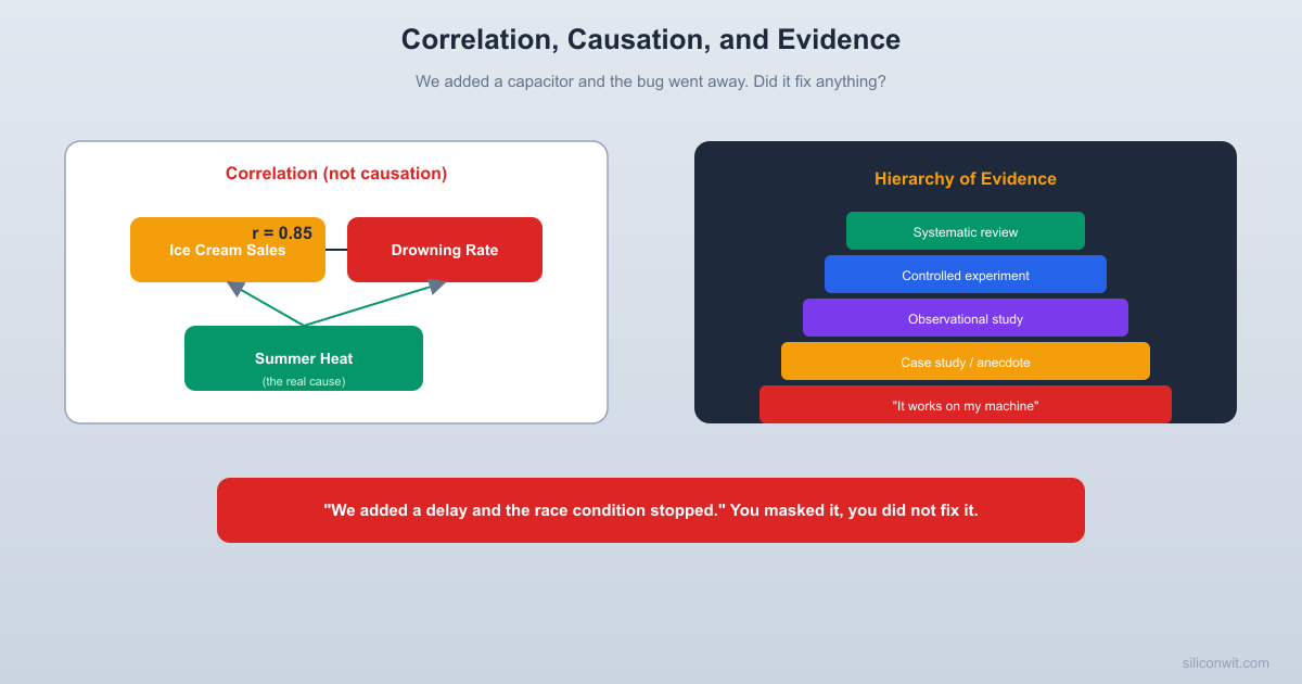
The classic example: ice cream sales and drowning rates both increase in summer. Ice cream does not cause drowning. Hot weather causes both. Temperature is the confounding variable.
Confounders in Engineering
Observed Correlation
Possible Confounder
Teams that write more tests have fewer bugs
More experienced teams write more tests AND write better code
PCBs manufactured on Tuesday have lower defect rates
The factory does maintenance on Monday night
Code reviewed by Alice has fewer issues
Alice reviews the modules she wrote, and she writes clean code
Projects using Language X ship faster
Companies choosing Language X tend to be startups with less bureaucracy
Devices with newer firmware have fewer field failures
Newer firmware is deployed on newer hardware that also has fewer defects
Engineers who use tool X produce cleaner designs
Engineers who care about clean designs tend to seek out better tools
The key question to ask when you see a correlation is: “What else could explain this?” If you can think of a plausible third variable that drives both the “cause” and the “effect,” you have found a potential confounder. Getting into the habit of asking this question is more valuable than any statistical technique.
This simulation generates ice cream sales and drowning incidents that are both driven by temperature (the hidden confounder). The two variables appear correlated, but once you account for temperature, the relationship vanishes.
confounding_variable_demo.py
import numpy as np
from scipy import stats
np.random.seed(42)
n_days =200
# Temperature is the confounder (in Celsius)
temperature = np.random.normal(loc=25,scale=8,size=n_days)
# Ice cream sales driven by temperature + noise
ice_cream =50+3.0* temperature + np.random.normal(0,10, n_days)
# Drowning incidents driven by temperature + noise
drowning =1.0+0.15* temperature + np.random.normal(0,1.5, n_days)
print(f"Partial correlation (temperature removed): r = {r_partial:.3f}, p = {p_partial:.6f}")
print(f"\nBefore controlling for temperature: strong correlation (r={r_raw:.3f})")
print(f"After controlling for temperature: correlation vanishes (r={r_partial:.3f})")
print(f"Temperature was the confounder all along.")
How to Deal With Confounders
List possible confounders. Before concluding that A causes B, brainstorm what else could explain the association.
Control for them. If you suspect team experience is a confounder, compare teams with similar experience levels.
Randomize. If possible, randomly assign subjects to conditions. Randomization tends to balance confounders across groups, even ones you did not think of.
Be honest. If you cannot control for confounders, say so. “A is correlated with B, but we have not controlled for C” is a much more honest statement than “A causes B.”
Controlled Experiments: Change One Variable at a Time
The single most powerful tool for establishing causation is the controlled experiment. The idea is simple: hold everything constant except the one thing you want to test.
If your embedded system crashes intermittently and you suspect the power supply, do not simultaneously swap the power supply, add bypass capacitors, change the clock speed, and update the firmware. You have no idea which change (if any) fixed the problem. Change the power supply and only the power supply. Test. If the problem persists, revert that change and try the next one.
The Scientific Method for Engineers
One Variable at a Time
Observe the symptom (system crashes every 20 minutes).
Form a hypothesis (the 3.3 V rail has excessive ripple).
Design a test that changes only one thing (swap to a known-good LDO regulator).
Predict the outcome if the hypothesis is correct (crashes should stop).
Run the test and observe.
If crashes stop, you have evidence (not proof) that the power supply was the issue. Swap back the original to confirm the crashes return.
This feels slow. It feels inefficient. You will be tempted to change three things at once “just to save time.” But when the problem does not go away after your multi-change intervention, you will have no idea which changes helped, which were neutral, and which might have introduced new problems.
When You Must Change Multiple Things
Sometimes you genuinely cannot change just one variable. The new firmware requires a different hardware configuration, for instance. In those cases, document every change you made, and be honest that you cannot attribute the outcome to any single change. You can say: “After updating the firmware and replacing the voltage regulator, the crashes stopped. We have not isolated which change was responsible.”
The Control Group Mindset
Even in everyday engineering work, you can adopt the control group mindset. When testing a new PCB layout revision, keep a few boards with the old layout for comparison. When deploying a software update, monitor a set of systems still running the old version. When trying a new soldering technique, solder half the boards the old way and half the new way.
The point is not to run a formal experiment every time. The point is to always have a baseline for comparison. Without a baseline, you cannot tell whether your results are good, bad, or unchanged.
A/B Testing: The Engineering Clinical Trial
A/B testing is the controlled experiment applied at scale. Instead of testing on one system, you run two versions simultaneously and compare results.
Software A/B Testing
You have two versions of a web page layout. Version A is the current design. Version B has a larger “Buy” button. You randomly assign 50% of users to each version and measure the click-through rate over a week. If version B gets significantly more clicks and the difference is statistically significant, you have evidence that the button size matters.
The key phrase is “randomly assign.” If you let users self-select into groups, the groups might differ in ways that confound the results. Random assignment is what makes A/B testing powerful: it tends to balance both known and unknown confounders across the groups.
Hardware A/B Testing
You can do this with hardware too. You have two PCB revisions: the original and one with an improved ground plane. Build 20 of each, run them through the same test suite, and compare failure rates. If revision B has substantially fewer failures, the ground plane improvement likely helped.
In hardware, randomization means testing both versions under the same conditions. Do not test all revision A boards in the morning and all revision B boards in the afternoon (temperature drift could confound the results). Alternate between the two revisions, or better yet, randomize the test order.
What Makes a Good A/B Test
Requirement
Why
Randomization
Ensures the two groups are comparable
Large enough sample
Small samples produce noisy results
Single variable changed
Otherwise you do not know what caused the difference
Controlled duration
Running until you “see a difference” biases results
Statistical significance test
Tells you whether the difference is real or just noise
Common A/B Testing Mistakes
One of the most common mistakes is “peeking”: checking the results every day and stopping the test as soon as one variant looks better. This introduces a statistical bias because random fluctuations can make one variant look temporarily better even when there is no real difference. Set a sample size and duration before you start, and do not change them partway through.
Another mistake is testing too many variants at once. If you test five different button colors, five font sizes, and three layouts simultaneously, you need an enormous sample to detect differences, and you risk finding “significant” results that are actually random noise (the multiple comparisons problem).
When A/B Testing Is Not Practical
Some engineering decisions cannot be A/B tested. You cannot build two bridges and see which one lasts longer. You cannot ship two different processor architectures in the same product. For these decisions, you rely on simulation, analysis, expert judgment, and historical data, while being honest that your evidence is weaker than a controlled experiment would provide.
Anecdotal Evidence vs. Systematic Evidence
“It works on my machine” is anecdotal evidence. It tells you that the software works in one specific environment with one specific configuration at one specific time. It tells you almost nothing about whether it will work on your machine, or on the production server, or next Tuesday.
Anecdotal evidence is not worthless. It can suggest hypotheses and point you in useful directions. But it should never be the basis for engineering decisions by itself.
The Hierarchy of Evidence
Not all evidence is created equal. Here is a rough hierarchy, from weakest to strongest:
Expert opinion. “I think this is the right approach because I have been doing this for 20 years.” Valuable, but subject to bias and limited experience.
Anecdotal evidence. “This worked for me on my last project.” A single data point, possibly unrepresentative.
Case study. “We documented what happened on this project in detail.” More rigorous than anecdote, but still a single instance.
Observational study. “We looked at 50 projects and found that teams using code review had 30% fewer production bugs.” Correlation, but not controlled for confounders.
Controlled experiment. “We randomly assigned 20 teams to use code review and 20 to skip it, holding everything else constant.” Much stronger evidence of causation.
Systematic review. “We analyzed 15 controlled experiments on code review practices and synthesized the results.” The gold standard: multiple independent studies pointing to the same conclusion.
Applying This in Practice
When someone makes a claim, mentally place it on this hierarchy. “Stack Overflow says this library is faster” is barely above anecdote. “We benchmarked both libraries on our hardware with our workload and library B is 2.3x faster (n=100 runs, p less than 0.01)” is a controlled experiment.
You do not need to run systematic reviews before choosing a library. But you should be aware of how strong your evidence is, and calibrate your confidence accordingly.
The next simulation shows how cherry-picking a single data point from a noisy upward trend can lead to the opposite conclusion. One person looks at a dip and declares “it is going down,” while the full trend tells a completely different story.
anecdotal_vs_trend.py
import numpy as np
np.random.seed(42)
n_months =24
months = np.arange(n_months)
# Clear upward trend with noise
trend =100+1.5* months
noise = np.random.normal(0,5, n_months)
data = trend + noise
# Find a noticeable dip (a point lower than its predecessor)
dips = np.where(np.diff(data)<-3)[0]+1# indices where data dropped
cherry_pick = dips[len(dips) //2] # pick a dip near the middle
print(f"Overall change (first to last): {total_change:+.1f}%\n")
print(f"Cherry-picked point (month {cherry_pick}): {local_change:+.1f}% drop from previous month")
print(f"\nAnecdotal claim: 'See, month {cherry_pick} dropped {abs(local_change):.1f}%! It is declining!'")
print(f"Full trend: 'The data rose {total_change:.1f}% over {n_months} months.'")
print(f"\nOne data point is not a trend. Always look at the full picture.")
The “N=1” Problem
Much of engineering practice is based on N=1 evidence: “we tried this on one project and it worked.” That is better than nothing, but it is weak evidence for generalizing. Maybe it worked because of specific circumstances on that project. Maybe it would have worked regardless of your choice. Maybe the next project has different constraints that make the same approach fail.
When you base a decision on N=1 evidence, acknowledge it. “This approach worked well on Project X, but we have not tested it more broadly” is honest. “This is the right approach because it worked on Project X” is overconfident.
Calibrating Confidence
A useful habit: after stating a claim, rate your confidence on a scale of 1 to 10. “I am about 3/10 confident this library handles edge cases correctly” forces you to be explicit about uncertainty. It also helps others understand how much weight to put on your recommendation.
“The Code Works When I Add a Delay”
This is one of the most common examples of mistaking correlation for causation in embedded systems. Your code crashes. You add a 10 ms delay somewhere. The crash goes away. You ship it.
What probably happened: you have a race condition. Two tasks (or an ISR and a main loop) are accessing the same data without proper synchronization. The delay changes the timing just enough that the race condition rarely triggers. You did not fix the bug. You hid it. And it will come back, probably at the worst possible time, in a demo, during a customer visit, or in a product that has already shipped.
Other Timing-Dependent “Fixes” That Mask Bugs
The delay trick is just one example of a broader pattern. Here are other common timing-dependent “fixes” that should make you suspicious:
“Fix”
What It Probably Masks
Adding volatile keyword
A compiler optimization that exposed a real synchronization bug
Reducing optimization level
Same as above; the bug is in the code, not the optimizer
Adding a print/log statement
The I/O slows things down enough to avoid a race condition
Increasing a buffer size
An off-by-one error or a boundary condition that was not handled
Restarting the service periodically
A memory leak or resource exhaustion
”Power cycle fixes it”
An initialization bug that only manifests after a warm restart
If your fix falls into one of these categories, you should keep investigating. The real bug is still there.
The problem comes back intermittently even with the fix.
The fix is timing-dependent (it works at 10 ms but not at 5 ms).
You cannot explain the root cause to a colleague.
Signs you actually fixed the bug:
You identified the root cause (e.g., unsynchronized access to a shared variable).
You understand why the fix works (e.g., you added a mutex that serializes access).
The fix is robust to timing changes (it works whether the system is fast or slow).
You can explain the mechanism to a colleague.
You can write a test that reproduces the original bug and verify the fix prevents it.
Thinking in Mechanisms
The difference between correlation and causation often comes down to whether you can describe a mechanism. A mechanism is a step-by-step causal chain explaining how A leads to B.
“Adding a bypass capacitor fixed the noise” is a correlation statement. “The MCU draws short current pulses during clock transitions, which caused voltage dips on the power rail. The bypass capacitor provides local charge storage, reducing the voltage dip below the MCU’s brown-out threshold” is a mechanism. Once you have a mechanism, you have a much stronger basis for believing that A actually caused B.
Questions That Reveal Mechanisms
When someone claims A caused B, ask:
How? What is the physical or logical pathway from A to B?
Why this amount? If A is proportional to B, the mechanism should explain the proportionality.
What would break it? If the mechanism is real, there should be conditions under which it would not work.
What else would the mechanism predict? A good mechanism makes predictions beyond the original observation. Test those predictions.
Building a Causal Diagram
A causal diagram (sometimes called a directed acyclic graph or DAG) is a visual tool for mapping out cause-and-effect relationships. Each variable is a node, and each arrow shows the direction of causation.
For the motor noise example:
Motor Running ──> Electromagnetic Interference ──> Noise on ADC Lines ──> Noisy Sensor Readings
^
Motor Running ──> Vibration ──> Loose Connector ────────┘
Drawing the diagram forces you to make your causal assumptions explicit. You might realize there are multiple pathways from cause to effect, and your proposed fix only addresses one of them.
Survivorship Bias
Survivorship bias occurs when you draw conclusions from only the successful cases, ignoring the failures. In engineering, this shows up constantly.
“Company X does not write unit tests and they are hugely successful.” How many companies skipped unit tests and failed quietly? You never hear about them because they are gone. You only see the survivors.
“This open-source project has no formal code review process and the code is excellent.” How many open-source projects without code review produced terrible code and died in obscurity? You only see the ones that succeeded despite the lack of process.
Recognizing Survivorship Bias
Whenever you see a pattern among successful examples, ask: “What about the failures?” If you only have data on the successes, your pattern might be meaningless. The failures might show the exact same pattern, which would mean the pattern is unrelated to success.
The Airplane Armor Story
During World War II, the military analyzed bullet holes in returning bombers and planned to add armor where the holes were concentrated. Statistician Abraham Wald pointed out the flaw: the planes that returned were the ones that survived being hit in those locations. The missing data was the planes that did not return, which were likely hit in the unarmored areas. The military should armor the places with no bullet holes on returning planes, because those were the locations where a hit was fatal.
This is one of the most famous examples of survivorship bias, and it is directly applicable to engineering. When you analyze failures, also consider what you are not seeing.
Simpson’s Paradox: When Aggregated Data Lies
Simpson’s paradox occurs when a trend that appears in several different groups of data reverses when the groups are combined. It sounds impossible, but it happens more often than you might expect.
A Software Example
Suppose you are comparing two compilers. Compiler A produces faster code on small programs and faster code on large programs. But when you average across all programs, Compiler B appears faster. How?
Program Size
Compiler A
Compiler B
Winner
Small (80% of tests)
10 ms avg
12 ms avg
A
Large (20% of tests)
100 ms avg
120 ms avg
A
Overall average
28 ms
33.6 ms… wait
Actually that example works out in A’s favor. The paradox arises when the groups have very different sizes and different proportions in each sample. Consider: team 1 runs mostly large programs, team 2 runs mostly small programs. When you combine their benchmarks without accounting for program size, the mix shifts and the apparent winner can flip.
The lesson: always look at the subgroups before trusting an aggregate statistic. If the trend reverses when you break the data down, the aggregate is misleading.
Why This Matters for Engineers
You might see overall failure rates for two manufacturing processes and conclude one is better. But if Process A is used mostly for simple boards and Process B for complex boards, the comparison is unfair. Break the data down by board complexity before drawing conclusions.
Bayesian Thinking for Engineers
Bayes’ theorem tells you how to update your beliefs when new evidence arrives. The intuition is simple: your confidence in a hypothesis should depend on how likely the evidence is if the hypothesis is true versus how likely the evidence is if the hypothesis is false.
A Practical Example
Your circuit board sometimes resets. You have two hypotheses:
Hypothesis A: Noisy power supply (prior probability: 60%, because this is a common issue)
You add a decoupling capacitor and the resets become less frequent but do not stop entirely. How should this evidence update your beliefs?
If the power supply were the problem, adding a cap would likely reduce but might not eliminate resets (probability of this evidence given H_A: 70%). If it were a firmware bug, adding a cap would have no effect on resets on average, but random variation might make it seem like they decreased (probability of this evidence given H_B: 20%).
Using Bayes’ rule informally: the evidence favors H_A (power supply) because it is much more likely under H_A than H_B. Your updated belief should shift toward the power supply hypothesis, but not fully, because H_B is not ruled out.
You do not need to compute exact probabilities in practice. The key insight is to ask: “How likely is this evidence under each hypothesis?” Evidence that is equally likely under both hypotheses tells you nothing. Evidence that is much more likely under one hypothesis is highly informative.
Pre-Test vs. Post-Test Probability
Before running a diagnostic test, you have a prior probability (your initial guess based on experience). After the test, you have a posterior probability (your updated belief). The strength of the update depends on how discriminating the test is.
A test that gives the same result regardless of the true cause is useless, even if it looks scientific. A test that gives different results depending on the cause is valuable. When choosing which diagnostic test to run next during debugging, ask: “Will this test’s result help me distinguish between my competing hypotheses?” If the answer is no, pick a different test.
Exercises
Spot the fallacy. A team reports: “After switching from C to Rust, our bug count dropped by 40%.” List three confounding variables that could explain this result without Rust’s memory safety being the cause.
Design a controlled experiment. Your colleague claims that code reviews catch more bugs than unit tests. Design an experiment to test this claim. What variables would you control? What would you measure? How would you handle confounders like developer experience?
Evaluate evidence strength. You are choosing between two RTOS options for a product. One option has a forum post saying “this RTOS is rock solid, we have used it for years.” The other has a published benchmark comparing latency and jitter across 1000 runs on your target hardware. Which is stronger evidence, and why?
Find the mechanism. Your sensor gives noisy readings when the motor is running and clean readings when the motor is off. Propose a causal mechanism (not just “the motor causes noise”) that explains the step-by-step physical pathway. Then propose a test that would confirm or refute your mechanism.
Survivorship bias. You read that successful startups in your industry rarely write detailed requirements documents. Should you skip requirements for your next project? What survivorship bias might be at play? What data would you need to make this decision properly?
Bayesian update. Your embedded device fails intermittently. You believe there is a 70% chance it is a hardware issue and a 30% chance it is a firmware issue. You run the same firmware on a different board and the failure does not occur. How should this evidence update your beliefs? What if the second board is a different revision with a slightly different layout?
Practical Takeaways
Questions to Ask About Any Claim
Before accepting that A caused B, ask these questions:
Is this just correlation, or is there a mechanism?
What confounders could explain the association?
Was a controlled experiment done, or is this observational?
How large is the sample? Could it be random variation?
Can the result be reproduced independently?
What would it look like if the claim were false?
These questions do not require advanced statistics. They require the habit of thinking carefully before accepting convenient explanations. That habit, more than any technical tool, is what separates rigorous engineers from ones who get fooled by coincidence.
Summary
Correlation is not causation, and every engineer needs to internalize that distinction. Just because a change preceded an improvement does not mean the change caused the improvement. Confounding variables lurk everywhere, creating the illusion of causal relationships. Controlled experiments, where you change one variable at a time and properly control for confounders, are the most reliable way to establish causation. When you cannot run a controlled experiment, be honest about the strength of your evidence. And always look for mechanisms: step-by-step causal chains that explain how and why something happens, not just that it happens.
Comments