Edge-Cloud Hybrid Architectures

Modified: Mar. 14, 2026

Published: Mar. 9, 2026

Running every inference on a cloud server introduces latency, bandwidth costs, and a single point of failure when the network drops. Running every inference on the edge device means you are limited to small models that sometimes lack the accuracy to handle ambiguous inputs. The hybrid approach combines both: the edge handles the easy cases instantly, the cloud handles the hard ones with a bigger model, and a retraining loop keeps the edge model improving over time. This lesson builds that complete system on hardware you already have from previous lessons. #EdgeCloud #TinyML #HybridAI

What We Are Building

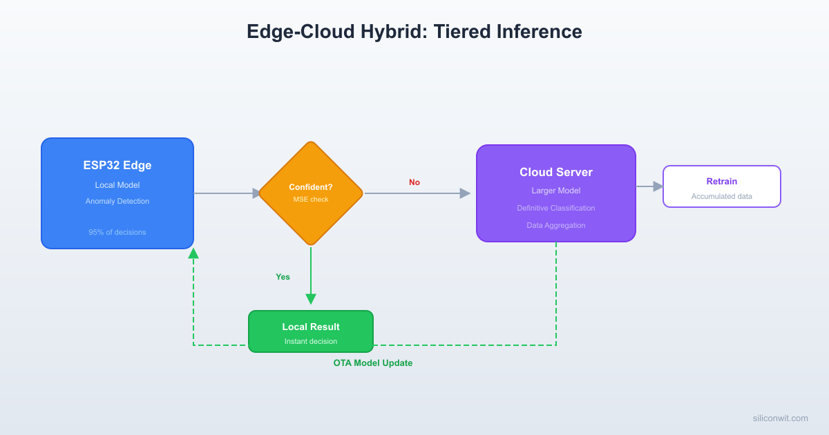
Edge-Cloud Hybrid Anomaly Detector

An ESP32 running the autoencoder from Lesson 7 (anomaly detection on motor vibration). When the reconstruction error falls clearly below or above the threshold, the ESP32 decides locally. When the error lands in an ambiguous zone near the threshold, the ESP32 sends the feature vector to a Python cloud server running a larger, more accurate model. The cloud returns a definitive classification. Periodically, the cloud retrains the edge model using accumulated escalated data, quantizes it, and pushes the updated .tflite to the ESP32 via HTTP OTA. An MQTT dashboard displays edge decisions, cloud escalations, model version, and device health.

System specifications:

Parameter	Value
Edge MCU	ESP32 DevKitC
Edge model	Autoencoder, ~12 KB int8 TFLite (from Lesson 7)
Cloud model	Larger autoencoder, ~200 KB float32 TensorFlow
Cloud server	Python FastAPI on a Linux host (PC, RPi 4, or VPS)
Escalation trigger	MSE in ambiguous zone between `low_threshold` and `high_threshold`
OTA transport	HTTP GET for `.tflite` file
Telemetry	MQTT (topics under `edge-ai/device/{id}/`)
Dashboard	Grafana or SiliconWit.io (covered in IoT Systems course)

Bill of Materials

Ref	Component	Quantity	Notes
U1	ESP32 DevKitC	1	Reuse from previous lessons
S1	MPU6050 breakout module	1	Reuse from Lesson 7
M1	Small DC motor or PC fan	1	Vibration source
	PC or Raspberry Pi 4	1	Cloud inference server
	Wi-Fi network	1	ESP32 and server on same network
	Breadboard + jumper wires	1 set

  OTA Model Update Sequence
  ──────────────────────────────────────────
  Cloud Server                  ESP32
  ────────────                  ─────
  Accumulate escalated data
       │
  Retrain edge model
       │
  Quantize to int8
       │
  Host model.tflite on HTTP
       │                   GET /model/v2.tflite
       ◄───────────────────────────┤
       │                           │
  Send .tflite bytes ─────────────►│
       │                           │
       │                   Write to flash partition
       │                   Verify checksum
       │                   Swap model pointer
       │                   Log: "Model v2 active"
       │                           │
       │                   Resume inference
       │                   with new model

  Edge-Cloud Hybrid Decision Flow
  ──────────────────────────────────────────
  Sensor Data ──► Edge Model (12 KB, ESP32)
                      │
                      ▼
              ┌───────────────┐
              │ MSE < low_thr │──► NORMAL
              │               │    (local decision)
              │ MSE > hi_thr  │──► ANOMALY
              │               │    (local decision)
              │ low < MSE < hi│──► UNCERTAIN
              └───────┬───────┘       │
                      │               │ escalate
                      │               ▼
                      │    Cloud Model (200 KB)
                      │        │
                      │        ▼
                      │    Definitive answer
                      │        │
                      │    OTA retrain loop:
                      │    accumulated data ──►
                      │    retrain edge model ──►
                      │    push .tflite via HTTP
                      ▼
               MQTT Dashboard

Architecture Overview

The system operates in three tiers. Each tier has a clear responsibility, and data flows upward only when the lower tier cannot handle the decision with sufficient confidence.

Tier 1: Edge Inference

The ESP32 collects a vibration window from the MPU6050 (100 samples at 200 Hz, 3 axes, yielding 300 values). It runs the small autoencoder and computes the mean squared error (MSE) between input and reconstruction. If the MSE is clearly below low_threshold, the input is classified as normal. If the MSE is clearly above high_threshold, the input is classified as anomalous. In both cases, the ESP32 acts immediately: toggling an LED, publishing an MQTT message, and moving to the next window. Approximately 95% of all inferences resolve at this tier.

Tier 2: Cloud Inference

When the MSE falls between low_threshold and high_threshold (the ambiguous zone), the ESP32 packages the 300-value feature vector as JSON and sends an HTTP POST to the cloud server. The server runs the same input through a larger autoencoder (wider layers, float32 precision) that is more accurate in the ambiguous region. The server returns a JSON response with the classification and confidence score. The ESP32 uses this result to make the final decision. This tier handles roughly 5% of inferences.

Tier 3: Cloud Retraining

The cloud server stores every escalated feature vector along with its final classification. Periodically (e.g., once per day, or after accumulating 500 new samples), a retraining script loads all accumulated data, retrains the edge autoencoder with the expanded dataset, quantizes the result to int8, and saves the new .tflite file to a directory served by HTTP. The next time the ESP32 checks for updates (on boot or on a timer), it downloads the new model, writes it to a dedicated flash partition, and reloads the TFLite Micro interpreter. Over time, the edge model’s ambiguous zone shrinks as it learns from the cases it previously could not handle.

Data Flow

The data flows through the system as follows. The ESP32 reads a vibration window from the MPU6050 over I2C. It runs the autoencoder and computes MSE. If the result is decisive, the ESP32 publishes the classification to MQTT topic edge-ai/device/{id}/inference and proceeds. If the result is ambiguous, the ESP32 posts the feature vector to http://{server}:8000/classify, receives the cloud classification, publishes both the edge MSE and cloud result to MQTT topic edge-ai/device/{id}/escalation, and proceeds. On a separate timer, the ESP32 sends an HTTP GET to http://{server}:8000/model/version to check for updates. If a new model version is available, it downloads the .tflite file, writes it to the model partition in flash, reinitializes the interpreter, and publishes the new model version to MQTT topic edge-ai/device/{id}/status.

Tiered Inference: When to Escalate

The core idea is to define a confidence zone around the anomaly threshold. Instead of a single threshold, you use two.

Zone	MSE Range	Decision	Actor
Normal	MSE < `low_threshold`	Normal (high confidence)	Edge
Ambiguous	`low_threshold` to `high_threshold`	Uncertain (escalate)	Cloud
Anomaly	MSE > `high_threshold`	Anomaly (high confidence)	Edge

You derive low_threshold and high_threshold from the training data distribution. If the mean training MSE is mu and the standard deviation is sigma, a reasonable starting point is:

low_threshold = mu + 2.0 * sigma
high_threshold = mu + 4.0 * sigma

This means anything within 2 sigma of the normal mean is definitely normal, anything beyond 4 sigma is definitely anomalous, and the zone between 2 and 4 sigma gets escalated. You can tune these multipliers based on your application’s tolerance for false positives vs false negatives.

ESP32 Tiered Decision Logic

The following code integrates into the inference loop from Lesson 7. After computing the MSE, instead of comparing against a single threshold, it routes through the three-zone logic.

#ifndef TIERED_INFERENCE_H
#define TIERED_INFERENCE_H

#include <stdbool.h>

typedef enum {
    DECISION_NORMAL,
    DECISION_ANOMALY,
    DECISION_UNCERTAIN
} inference_decision_t;

typedef struct {
    float mse;
    inference_decision_t decision;
    bool escalated;
    float cloud_confidence;
    int cloud_classification;  // 0=normal, 1=anomaly, -1=not escalated
} inference_result_t;

// Thresholds (set from training data statistics)
extern float g_low_threshold;
extern float g_high_threshold;

inference_decision_t classify_mse(float mse);

#endif

#include "tiered_inference.h"

float g_low_threshold = 0.015f;   // mu + 2*sigma (example values)
float g_high_threshold = 0.045f;  // mu + 4*sigma (example values)

inference_decision_t classify_mse(float mse)
{
    if (mse < g_low_threshold) {
        return DECISION_NORMAL;
    } else if (mse > g_high_threshold) {
        return DECISION_ANOMALY;
    } else {
        return DECISION_UNCERTAIN;
    }
}

The main inference loop uses this function to decide whether to act locally or escalate.

// In the main inference task
void inference_task(void *pvParameters)
{
    float input_buffer[300];
    float output_buffer[300];
    inference_result_t result;

    while (1) {
        // Collect vibration window (from Lesson 7)
        collect_vibration_window(input_buffer, 100, 3);

        // Run local autoencoder
        run_autoencoder_inference(input_buffer, output_buffer, 300);

        // Compute MSE
        result.mse = compute_mse(input_buffer, output_buffer, 300);
        result.decision = classify_mse(result.mse);
        result.escalated = false;
        result.cloud_confidence = 0.0f;
        result.cloud_classification = -1;

        if (result.decision == DECISION_UNCERTAIN) {
            // Escalate to cloud
            result.escalated = true;
            esp_err_t err = escalate_to_cloud(input_buffer, 300, &result);
            if (err != ESP_OK) {
                // Cloud unreachable: fall back to nearest threshold
                result.decision = (result.mse < (g_low_threshold + g_high_threshold) / 2.0f)
                    ? DECISION_NORMAL : DECISION_ANOMALY;
                ESP_LOGW("INFER", "Cloud unreachable, fallback decision: %d", result.decision);
            }
        }

        // Act on decision
        handle_decision(&result);

        // Publish to MQTT
        publish_inference_result(&result);

        vTaskDelay(pdMS_TO_TICKS(500));
    }
}

Notice the fallback logic: if the cloud server is unreachable, the ESP32 picks the closer threshold rather than blocking. This ensures the system never stalls waiting for a network response.

Cloud Inference Server

The cloud server is a Python FastAPI application. It loads a larger autoencoder (trained on the same vibration data but with wider layers and float32 precision) and exposes two endpoints: /classify for inference and /model/version for OTA version checking.

Server Setup

Install the dependencies: pip install fastapi uvicorn tensorflow numpy
Train the larger cloud model (see the retraining section below) or use an expanded version of the Lesson 7 autoencoder
Place the saved model in a models/ directory
Run the server: uvicorn cloud_server:app --host 0.0.0.0 --port 8000

Full Server Code

import json
import time
import logging
from pathlib import Path

import numpy as np
import tensorflow as tf
from fastapi import FastAPI, HTTPException
from pydantic import BaseModel

logging.basicConfig(level=logging.INFO)
logger = logging.getLogger("cloud_server")

app = FastAPI(title="Edge-Cloud Hybrid Inference Server")

# Configuration
CLOUD_MODEL_PATH = "models/cloud_autoencoder"
EDGE_MODEL_DIR = "models/edge"
ESCALATION_LOG = "data/escalations.jsonl"
ANOMALY_THRESHOLD = 0.025  # Cloud model threshold (tighter than edge)
INPUT_SIZE = 300

# Load cloud model
cloud_model = tf.keras.models.load_model(CLOUD_MODEL_PATH)
logger.info(f"Loaded cloud model from {CLOUD_MODEL_PATH}")

# Track edge model version
edge_model_version_file = Path(EDGE_MODEL_DIR) / "version.txt"
if edge_model_version_file.exists():
    EDGE_MODEL_VERSION = int(edge_model_version_file.read_text().strip())
else:
    EDGE_MODEL_VERSION = 1

class FeatureVector(BaseModel):
    device_id: str
    features: list[float]
    edge_mse: float

class ClassificationResponse(BaseModel):
    classification: int  # 0=normal, 1=anomaly
    confidence: float
    cloud_mse: float
    model_version: int

class ModelVersionResponse(BaseModel):
    version: int
    filename: str
    size_bytes: int

@app.post("/classify", response_model=ClassificationResponse)
async def classify(data: FeatureVector):
    if len(data.features) != INPUT_SIZE:
        raise HTTPException(
            status_code=400,
            detail=f"Expected {INPUT_SIZE} features, got {len(data.features)}"
        )

    # Run cloud model inference
    input_array = np.array(data.features, dtype=np.float32).reshape(1, INPUT_SIZE)
    reconstruction = cloud_model.predict(input_array, verbose=0)
    mse = float(np.mean((input_array - reconstruction) ** 2))

    classification = 1 if mse > ANOMALY_THRESHOLD else 0
    # Confidence: how far from threshold (normalized)
    distance = abs(mse - ANOMALY_THRESHOLD)
    confidence = min(distance / ANOMALY_THRESHOLD, 1.0)

    # Log the escalation for future retraining
    log_entry = {
        "timestamp": time.time(),
        "device_id": data.device_id,
        "features": data.features,
        "edge_mse": data.edge_mse,
        "cloud_mse": mse,
        "classification": classification
    }
    Path("data").mkdir(exist_ok=True)
    with open(ESCALATION_LOG, "a") as f:
        f.write(json.dumps(log_entry) + "\n")

    logger.info(
        f"Device {data.device_id}: edge_mse={data.edge_mse:.6f}, "
        f"cloud_mse={mse:.6f}, class={classification}, conf={confidence:.3f}"
    )

    return ClassificationResponse(
        classification=classification,
        confidence=confidence,
        cloud_mse=mse,
        model_version=EDGE_MODEL_VERSION
    )

@app.get("/model/version", response_model=ModelVersionResponse)
async def get_model_version():
    tflite_path = Path(EDGE_MODEL_DIR) / "model.tflite"
    if not tflite_path.exists():
        raise HTTPException(status_code=404, detail="No edge model available")

    return ModelVersionResponse(
        version=EDGE_MODEL_VERSION,
        filename="model.tflite",
        size_bytes=tflite_path.stat().st_size
    )

@app.get("/model/download")
async def download_model():
    from fastapi.responses import FileResponse
    tflite_path = Path(EDGE_MODEL_DIR) / "model.tflite"
    if not tflite_path.exists():
        raise HTTPException(status_code=404, detail="No edge model available")
    return FileResponse(
        path=str(tflite_path),
        media_type="application/octet-stream",
        filename="model.tflite"
    )

The server logs every escalated feature vector to a JSONL file. This file becomes the training data for the retraining pipeline. Each line contains the raw features, the edge MSE that triggered escalation, and the cloud model’s final classification.

ESP32 Cloud Escalation

When the edge model returns an uncertain MSE, the ESP32 needs to send the feature vector to the cloud and parse the response. This uses the ESP-IDF HTTP client library.

#include <string.h>
#include "esp_log.h"
#include "esp_http_client.h"
#include "cJSON.h"
#include "tiered_inference.h"

static const char *TAG = "CLOUD";

// Configuration
#define CLOUD_SERVER_URL "http://192.168.1.100:8000/classify"
#define DEVICE_ID "esp32-vibration-001"
#define HTTP_TIMEOUT_MS 5000
#define MAX_RESPONSE_SIZE 512

static char response_buffer[MAX_RESPONSE_SIZE];
static int response_len = 0;

static esp_err_t http_event_handler(esp_http_client_event_t *evt)
{
    switch (evt->event_id) {
    case HTTP_EVENT_ON_DATA:
        if (response_len + evt->data_len < MAX_RESPONSE_SIZE) {
            memcpy(response_buffer + response_len, evt->data, evt->data_len);
            response_len += evt->data_len;
        }
        break;
    default:
        break;
    }
    return ESP_OK;
}

esp_err_t escalate_to_cloud(const float *features, int num_features,
                            inference_result_t *result)
{
    esp_err_t ret = ESP_FAIL;
    response_len = 0;
    memset(response_buffer, 0, MAX_RESPONSE_SIZE);

    // Build JSON payload
    cJSON *root = cJSON_CreateObject();
    cJSON_AddStringToObject(root, "device_id", DEVICE_ID);
    cJSON_AddNumberToObject(root, "edge_mse", (double)result->mse);

    cJSON *feat_array = cJSON_CreateFloatArray(features, num_features);
    cJSON_AddItemToObject(root, "features", feat_array);

    char *post_data = cJSON_PrintUnformatted(root);
    cJSON_Delete(root);

    if (post_data == NULL) {
        ESP_LOGE(TAG, "Failed to serialize JSON");
        return ESP_ERR_NO_MEM;
    }

    ESP_LOGI(TAG, "Escalating to cloud, payload size: %d bytes", strlen(post_data));

    // Configure HTTP client
    esp_http_client_config_t config = {
        .url = CLOUD_SERVER_URL,
        .method = HTTP_METHOD_POST,
        .timeout_ms = HTTP_TIMEOUT_MS,
        .event_handler = http_event_handler,
    };

    esp_http_client_handle_t client = esp_http_client_init(&config);
    esp_http_client_set_header(client, "Content-Type", "application/json");
    esp_http_client_set_post_field(client, post_data, strlen(post_data));

    esp_err_t err = esp_http_client_perform(client);
    if (err != ESP_OK) {
        ESP_LOGE(TAG, "HTTP POST failed: %s", esp_err_to_name(err));
        goto cleanup;
    }

    int status = esp_http_client_get_status_code(client);
    if (status != 200) {
        ESP_LOGE(TAG, "Cloud returned status %d", status);
        goto cleanup;
    }

    // Parse response
    response_buffer[response_len] = '\0';
    cJSON *resp = cJSON_Parse(response_buffer);
    if (resp == NULL) {
        ESP_LOGE(TAG, "Failed to parse cloud response");
        goto cleanup;
    }

    cJSON *classification = cJSON_GetObjectItem(resp, "classification");
    cJSON *confidence = cJSON_GetObjectItem(resp, "confidence");
    cJSON *cloud_mse = cJSON_GetObjectItem(resp, "cloud_mse");

    if (classification && confidence) {
        result->cloud_classification = classification->valueint;
        result->cloud_confidence = (float)confidence->valuedouble;
        result->decision = (classification->valueint == 1)
            ? DECISION_ANOMALY : DECISION_NORMAL;

        ESP_LOGI(TAG, "Cloud decision: %s (confidence=%.3f, cloud_mse=%.6f)",
                 classification->valueint ? "ANOMALY" : "NORMAL",
                 confidence->valuedouble,
                 cloud_mse ? cloud_mse->valuedouble : 0.0);
        ret = ESP_OK;
    }

    cJSON_Delete(resp);

cleanup:
    esp_http_client_cleanup(client);
    free(post_data);
    return ret;
}

The key design choices here are the 5-second timeout (long enough for a Wi-Fi round trip, short enough to avoid blocking the inference loop) and the graceful degradation when the cloud is unreachable. The caller in inference_task handles the fallback to threshold-based classification.

OTA Model Updates

The most powerful aspect of a hybrid architecture is the ability to improve the edge model over time without physically touching the device. This section covers how to structure the ESP32 firmware so that the TFLite model is loaded from a flash partition rather than compiled into the binary, enabling updates without reflashing the entire firmware.

Partition Table

Add a custom partition for storing the model. Create a file called partitions.csv in your ESP-IDF project root.

# ESP-IDF Partition Table for OTA Model Updates
# Name,     Type, SubType, Offset,   Size,     Flags
nvs,        data, nvs,     0x9000,   0x6000,
phy_init,   data, phy,     0xf000,   0x1000,
factory,    app,  factory, 0x10000,  0x1E0000,
model,      data, fat,     0x1F0000, 0x10000,

The model partition is 64 KB, which is more than enough for a 12 KB quantized autoencoder with room to grow. Set the partition table in sdkconfig:

CONFIG_PARTITION_TABLE_CUSTOM=y
CONFIG_PARTITION_TABLE_CUSTOM_FILENAME="partitions.csv"

Writing and Reading the Model from Flash

#include <string.h>
#include "esp_log.h"
#include "esp_partition.h"
#include "model_storage.h"

static const char *TAG = "MODEL_STORE";

// Model header stored at the beginning of the partition
typedef struct {
    uint32_t magic;        // 0x4D4F444C ("MODL")
    uint32_t version;
    uint32_t model_size;
    uint32_t checksum;     // Simple CRC32
} model_header_t;

#define MODEL_MAGIC 0x4D4F444C
#define MODEL_PARTITION_LABEL "model"

static const esp_partition_t *get_model_partition(void)
{
    return esp_partition_find_first(
        ESP_PARTITION_TYPE_DATA,
        ESP_PARTITION_SUBTYPE_DATA_FAT,
        MODEL_PARTITION_LABEL
    );
}

static uint32_t compute_checksum(const uint8_t *data, size_t len)
{
    uint32_t crc = 0xFFFFFFFF;
    for (size_t i = 0; i < len; i++) {
        crc ^= data[i];
        for (int j = 0; j < 8; j++) {
            crc = (crc >> 1) ^ (0xEDB88320 & -(crc & 1));
        }
    }
    return ~crc;
}

esp_err_t model_storage_write(const uint8_t *model_data, size_t model_size,
                               uint32_t version)
{
    const esp_partition_t *part = get_model_partition();
    if (part == NULL) {
        ESP_LOGE(TAG, "Model partition not found");
        return ESP_ERR_NOT_FOUND;
    }

    if (sizeof(model_header_t) + model_size > part->size) {
        ESP_LOGE(TAG, "Model too large: %d bytes (partition: %d bytes)",
                 model_size, part->size);
        return ESP_ERR_INVALID_SIZE;
    }

    // Erase partition
    esp_err_t err = esp_partition_erase_range(part, 0, part->size);
    if (err != ESP_OK) {
        ESP_LOGE(TAG, "Failed to erase partition: %s", esp_err_to_name(err));
        return err;
    }

    // Write header
    model_header_t header = {
        .magic = MODEL_MAGIC,
        .version = version,
        .model_size = model_size,
        .checksum = compute_checksum(model_data, model_size)
    };

    err = esp_partition_write(part, 0, &header, sizeof(header));
    if (err != ESP_OK) {
        ESP_LOGE(TAG, "Failed to write header: %s", esp_err_to_name(err));
        return err;
    }

    // Write model data
    err = esp_partition_write(part, sizeof(header), model_data, model_size);
    if (err != ESP_OK) {
        ESP_LOGE(TAG, "Failed to write model: %s", esp_err_to_name(err));
        return err;
    }

    ESP_LOGI(TAG, "Wrote model v%lu (%lu bytes) to flash", version, model_size);
    return ESP_OK;
}

esp_err_t model_storage_read(uint8_t *buffer, size_t buffer_size,
                              uint32_t *version, size_t *model_size)
{
    const esp_partition_t *part = get_model_partition();
    if (part == NULL) {
        ESP_LOGE(TAG, "Model partition not found");
        return ESP_ERR_NOT_FOUND;
    }

    // Read header
    model_header_t header;
    esp_err_t err = esp_partition_read(part, 0, &header, sizeof(header));
    if (err != ESP_OK) return err;

    if (header.magic != MODEL_MAGIC) {
        ESP_LOGW(TAG, "No valid model in flash (bad magic)");
        return ESP_ERR_NOT_FOUND;
    }

    if (header.model_size > buffer_size) {
        ESP_LOGE(TAG, "Buffer too small: need %lu, have %d",
                 header.model_size, buffer_size);
        return ESP_ERR_INVALID_SIZE;
    }

    // Read model data
    err = esp_partition_read(part, sizeof(header), buffer, header.model_size);
    if (err != ESP_OK) return err;

    // Verify checksum
    uint32_t crc = compute_checksum(buffer, header.model_size);
    if (crc != header.checksum) {
        ESP_LOGE(TAG, "Checksum mismatch: expected 0x%08lX, got 0x%08lX",
                 header.checksum, crc);
        return ESP_ERR_INVALID_CRC;
    }

    *version = header.version;
    *model_size = header.model_size;
    ESP_LOGI(TAG, "Loaded model v%lu (%lu bytes) from flash", *version, *model_size);
    return ESP_OK;
}

uint32_t model_storage_get_version(void)
{
    const esp_partition_t *part = get_model_partition();
    if (part == NULL) return 0;

    model_header_t header;
    if (esp_partition_read(part, 0, &header, sizeof(header)) != ESP_OK) return 0;
    if (header.magic != MODEL_MAGIC) return 0;

    return header.version;
}

OTA Download and Update on ESP32

The ESP32 periodically checks the cloud server for a new model version. If a newer version is available, it downloads the .tflite file and writes it to the model partition.

#include <string.h>
#include "esp_log.h"
#include "esp_http_client.h"
#include "cJSON.h"
#include "model_storage.h"

static const char *TAG = "OTA_MODEL";

#define VERSION_URL "http://192.168.1.100:8000/model/version"
#define DOWNLOAD_URL "http://192.168.1.100:8000/model/download"
#define MAX_MODEL_SIZE (64 * 1024)

// Callback reference for interpreter reload
extern void reload_tflite_interpreter(const uint8_t *model_data, size_t model_size);

static uint8_t download_buffer[MAX_MODEL_SIZE];

static int check_remote_version(void)
{
    char resp_buf[256] = {0};
    int resp_len = 0;

    esp_http_client_config_t config = {
        .url = VERSION_URL,
        .timeout_ms = 5000,
    };

    esp_http_client_handle_t client = esp_http_client_init(&config);
    esp_err_t err = esp_http_client_open(client, 0);
    if (err != ESP_OK) {
        esp_http_client_cleanup(client);
        return -1;
    }

    int content_length = esp_http_client_fetch_headers(client);
    if (content_length > 0 && content_length < sizeof(resp_buf)) {
        resp_len = esp_http_client_read(client, resp_buf, content_length);
    }
    esp_http_client_close(client);
    esp_http_client_cleanup(client);

    if (resp_len <= 0) return -1;

    resp_buf[resp_len] = '\0';
    cJSON *json = cJSON_Parse(resp_buf);
    if (json == NULL) return -1;

    cJSON *version = cJSON_GetObjectItem(json, "version");
    int v = (version != NULL) ? version->valueint : -1;
    cJSON_Delete(json);
    return v;
}

static esp_err_t download_model(size_t *downloaded_size)
{
    esp_http_client_config_t config = {
        .url = DOWNLOAD_URL,
        .timeout_ms = 15000,
    };

    esp_http_client_handle_t client = esp_http_client_init(&config);
    esp_err_t err = esp_http_client_open(client, 0);
    if (err != ESP_OK) {
        esp_http_client_cleanup(client);
        return err;
    }

    int content_length = esp_http_client_fetch_headers(client);
    if (content_length <= 0 || content_length > MAX_MODEL_SIZE) {
        ESP_LOGE(TAG, "Invalid model size: %d", content_length);
        esp_http_client_close(client);
        esp_http_client_cleanup(client);
        return ESP_ERR_INVALID_SIZE;
    }

    int total_read = 0;
    while (total_read < content_length) {
        int read_len = esp_http_client_read(
            client,
            (char *)download_buffer + total_read,
            content_length - total_read
        );
        if (read_len <= 0) break;
        total_read += read_len;
    }

    esp_http_client_close(client);
    esp_http_client_cleanup(client);

    if (total_read != content_length) {
        ESP_LOGE(TAG, "Incomplete download: got %d of %d", total_read, content_length);
        return ESP_FAIL;
    }

    *downloaded_size = (size_t)total_read;
    ESP_LOGI(TAG, "Downloaded model: %d bytes", total_read);
    return ESP_OK;
}

void ota_model_update_task(void *pvParameters)
{
    while (1) {
        // Check every 30 minutes
        vTaskDelay(pdMS_TO_TICKS(30 * 60 * 1000));

        uint32_t local_version = model_storage_get_version();
        int remote_version = check_remote_version();

        if (remote_version <= 0 || (uint32_t)remote_version <= local_version) {
            ESP_LOGI(TAG, "No update available (local: v%lu, remote: v%d)",
                     local_version, remote_version);
            continue;
        }

        ESP_LOGI(TAG, "New model available: v%d (current: v%lu)",
                 remote_version, local_version);

        size_t model_size = 0;
        esp_err_t err = download_model(&model_size);
        if (err != ESP_OK) {
            ESP_LOGE(TAG, "Download failed: %s", esp_err_to_name(err));
            continue;
        }

        err = model_storage_write(download_buffer, model_size, (uint32_t)remote_version);
        if (err != ESP_OK) {
            ESP_LOGE(TAG, "Flash write failed: %s", esp_err_to_name(err));
            continue;
        }

        // Reload the interpreter with the new model
        reload_tflite_interpreter(download_buffer, model_size);

        ESP_LOGI(TAG, "Model updated to v%d, interpreter reloaded", remote_version);
    }
}

Reloading the TFLite Micro Interpreter

When a new model is written to flash, the interpreter must be reinitialized. The following function replaces the model pointer and rebuilds the interpreter.

// interpreter_reload.c (C++ file in practice, as TFLite Micro uses C++)
#include "tensorflow/lite/micro/micro_interpreter.h"
#include "tensorflow/lite/micro/micro_mutable_op_resolver.h"
#include "tensorflow/lite/schema/schema_generated.h"

static const int kTensorArenaSize = 32 * 1024;
static uint8_t tensor_arena[kTensorArenaSize];
static tflite::MicroInterpreter *interpreter = nullptr;
static uint8_t interpreter_buf[sizeof(tflite::MicroInterpreter)];

// Op resolver: initialized once at file scope
static tflite::MicroMutableOpResolver<4> resolver;
static bool resolver_initialized = false;

// Fallback: compiled-in model for first boot
extern const unsigned char g_default_model[];
extern const unsigned int g_default_model_len;

void reload_tflite_interpreter(const uint8_t *model_data, size_t model_size)
{
    const tflite::Model *model = tflite::GetModel(model_data);
    if (model->version() != TFLITE_SCHEMA_VERSION) {
        printf("Model schema version mismatch: %lu vs %lu\n",
               model->version(), TFLITE_SCHEMA_VERSION);
        return;
    }

    // Initialize the resolver once
    if (!resolver_initialized) {
        resolver.AddFullyConnected();
        resolver.AddRelu();
        resolver.AddReshape();
        resolver.AddQuantize();
        resolver_initialized = true;
    }

    // Destroy old interpreter if it exists
    if (interpreter) {
        interpreter->~MicroInterpreter();
    }

    // Construct a new interpreter in the pre-allocated buffer
    interpreter = new (interpreter_buf) tflite::MicroInterpreter(
        model, resolver, tensor_arena, kTensorArenaSize);

    if (interpreter->AllocateTensors() != kTfLiteOk) {
        printf("AllocateTensors failed for new model\n");
        interpreter->~MicroInterpreter();
        interpreter = nullptr;
        return;
    }

    printf("Interpreter reloaded with new model (%u bytes)\n",
           (unsigned)model_size);
}

On first boot, if no model is found in the flash partition, the firmware falls back to the compiled-in default model. After the first OTA update, subsequent boots load from flash.

Cloud Retraining Pipeline

The retraining script runs on the cloud server (manually or as a cron job). It reads all escalated feature vectors from the JSONL log, combines them with the original training data, retrains the edge autoencoder, quantizes it to int8, and saves the new .tflite file.

import json
import numpy as np
import tensorflow as tf
from pathlib import Path

# Configuration
ESCALATION_LOG = "data/escalations.jsonl"
ORIGINAL_TRAINING_DATA = "data/normal_vibration_training.npy"
EDGE_MODEL_DIR = "models/edge"
INPUT_SIZE = 300
MIN_NEW_SAMPLES = 50  # Minimum escalations before retraining

def load_escalated_data(log_path):
    """Load feature vectors from the escalation log."""
    features = []
    labels = []
    with open(log_path, "r") as f:
        for line in f:
            entry = json.loads(line.strip())
            features.append(entry["features"])
            labels.append(entry["classification"])
    return np.array(features, dtype=np.float32), np.array(labels)

def build_edge_autoencoder(input_size):
    """Build the edge autoencoder architecture (must match ESP32 expectations)."""
    encoder_input = tf.keras.Input(shape=(input_size,))
    x = tf.keras.layers.Dense(64, activation="relu")(encoder_input)
    encoded = tf.keras.layers.Dense(16, activation="relu")(x)
    x = tf.keras.layers.Dense(64, activation="relu")(encoded)
    decoded = tf.keras.layers.Dense(input_size, activation="linear")(x)

    autoencoder = tf.keras.Model(encoder_input, decoded)
    autoencoder.compile(optimizer="adam", loss="mse")
    return autoencoder

def quantize_and_export(model, representative_data, output_path):
    """Convert to int8 TFLite with full integer quantization."""
    converter = tf.lite.TFLiteConverter.from_keras_model(model)
    converter.optimizations = [tf.lite.Optimize.DEFAULT]

    def representative_dataset():
        for i in range(min(200, len(representative_data))):
            yield [representative_data[i:i+1].astype(np.float32)]

    converter.representative_dataset = representative_dataset
    converter.target_spec.supported_ops = [tf.lite.OpsSet.TFLITE_BUILTINS_INT8]
    converter.inference_input_type = tf.int8
    converter.inference_output_type = tf.int8

    tflite_model = converter.convert()

    Path(output_path).parent.mkdir(parents=True, exist_ok=True)
    with open(output_path, "wb") as f:
        f.write(tflite_model)

    print(f"Exported quantized model: {len(tflite_model)} bytes -> {output_path}")
    return tflite_model

def main():
    # Load original training data (normal samples only)
    original_data = np.load(ORIGINAL_TRAINING_DATA)
    print(f"Original training data: {original_data.shape}")

    # Load escalated data
    if not Path(ESCALATION_LOG).exists():
        print("No escalation log found. Nothing to retrain.")
        return

    escalated_features, escalated_labels = load_escalated_data(ESCALATION_LOG)
    print(f"Escalated samples: {len(escalated_features)}")

    if len(escalated_features) < MIN_NEW_SAMPLES:
        print(f"Only {len(escalated_features)} escalations (need {MIN_NEW_SAMPLES}). Skipping.")
        return

    # Use only the normal escalated samples for autoencoder training
    # (anomalous samples teach the model what NOT to reconstruct)
    normal_escalated = escalated_features[escalated_labels == 0]
    print(f"Normal escalated samples added to training: {len(normal_escalated)}")

    # Combine original and new normal data
    training_data = np.concatenate([original_data, normal_escalated], axis=0)
    np.random.shuffle(training_data)
    print(f"Combined training set: {training_data.shape}")

    # Split for validation
    split_idx = int(0.9 * len(training_data))
    train_set = training_data[:split_idx]
    val_set = training_data[split_idx:]

    # Build and train
    model = build_edge_autoencoder(INPUT_SIZE)
    model.fit(
        train_set, train_set,
        validation_data=(val_set, val_set),
        epochs=100,
        batch_size=32,
        callbacks=[
            tf.keras.callbacks.EarlyStopping(
                monitor="val_loss", patience=10, restore_best_weights=True
            )
        ],
        verbose=1
    )

    # Compute new thresholds
    reconstructions = model.predict(training_data, verbose=0)
    mse_values = np.mean((training_data - reconstructions) ** 2, axis=1)
    mu = np.mean(mse_values)
    sigma = np.std(mse_values)
    print(f"New threshold stats: mu={mu:.6f}, sigma={sigma:.6f}")
    print(f"Suggested low_threshold: {mu + 2*sigma:.6f}")
    print(f"Suggested high_threshold: {mu + 4*sigma:.6f}")

    # Read current version and increment
    version_file = Path(EDGE_MODEL_DIR) / "version.txt"
    if version_file.exists():
        current_version = int(version_file.read_text().strip())
    else:
        current_version = 0
    new_version = current_version + 1

    # Quantize and export
    tflite_path = Path(EDGE_MODEL_DIR) / "model.tflite"
    quantize_and_export(model, training_data, str(tflite_path))

    # Update version file
    version_file.write_text(str(new_version))
    print(f"Model version updated to v{new_version}")

    # Save threshold config for reference
    threshold_config = {
        "version": new_version,
        "mu": float(mu),
        "sigma": float(sigma),
        "low_threshold": float(mu + 2 * sigma),
        "high_threshold": float(mu + 4 * sigma),
        "training_samples": len(training_data),
        "escalated_samples_used": len(normal_escalated)
    }
    config_path = Path(EDGE_MODEL_DIR) / "threshold_config.json"
    with open(config_path, "w") as f:
        json.dump(threshold_config, f, indent=2)
    print(f"Threshold config saved to {config_path}")

    # Archive the processed escalation log
    archive_path = Path("data") / f"escalations_v{new_version}.jsonl"
    Path(ESCALATION_LOG).rename(archive_path)
    print(f"Escalation log archived to {archive_path}")

if __name__ == "__main__":
    main()

After running this script, the new model.tflite is immediately available at the /model/download endpoint. The next time any ESP32 device checks for updates, it will download and deploy the improved model.

Retraining Workflow

Escalated feature vectors accumulate in data/escalations.jsonl as the ESP32 devices encounter ambiguous cases
Run python retrain_edge_model.py manually, or schedule it as a daily cron job
The script combines original training data with newly collected normal samples
After training, it quantizes the model to int8 and increments the version number
ESP32 devices detect the new version on their next check cycle (every 30 minutes) and download the update automatically

MQTT Dashboard Integration

The ESP32 publishes all decisions, escalations, and system health to MQTT topics. This integrates directly with the MQTT broker and Grafana dashboards covered in the IoT Systems course.

Topic Hierarchy

edge-ai/
  device/
    {device_id}/
      inference       # Every local decision
      escalation      # Cloud escalation events
      status          # Model version, uptime, health
      ota             # OTA update events

JSON Payloads

Each message uses a consistent JSON structure with a timestamp, making it straightforward to parse in Grafana or any MQTT subscriber.

Inference result (local decision):

{
  "ts": 1741500000,
  "mse": 0.0082,
  "decision": "normal",
  "source": "edge",
  "model_version": 3
}

Escalation event:

{
  "ts": 1741500015,
  "edge_mse": 0.0312,
  "cloud_mse": 0.0289,
  "cloud_decision": "normal",
  "cloud_confidence": 0.87,
  "latency_ms": 142,
  "model_version": 3
}

Status heartbeat (every 60 seconds):

{
  "ts": 1741500060,
  "model_version": 3,
  "uptime_s": 86400,
  "total_inferences": 172800,
  "edge_decisions": 164160,
  "escalations": 8640,
  "free_heap": 45320,
  "wifi_rssi": -62
}

OTA update event:

{
  "ts": 1741500120,
  "event": "model_updated",
  "old_version": 2,
  "new_version": 3,
  "model_size": 12480,
  "download_ms": 850
}

ESP32 MQTT Publishing Code

#include <stdio.h>
#include <string.h>
#include <time.h>
#include "esp_log.h"
#include "esp_wifi.h"
#include "mqtt_client.h"
#include "cJSON.h"
#include "tiered_inference.h"
#include "model_storage.h"

static const char *TAG = "MQTT_PUB";
static esp_mqtt_client_handle_t mqtt_client = NULL;

#define DEVICE_ID "esp32-vibration-001"
#define TOPIC_INFERENCE   "edge-ai/device/" DEVICE_ID "/inference"
#define TOPIC_ESCALATION  "edge-ai/device/" DEVICE_ID "/escalation"
#define TOPIC_STATUS      "edge-ai/device/" DEVICE_ID "/status"
#define TOPIC_OTA         "edge-ai/device/" DEVICE_ID "/ota"

// Counters for status reporting
static uint32_t total_inferences = 0;
static uint32_t edge_decisions = 0;
static uint32_t escalation_count = 0;

void mqtt_publish_init(esp_mqtt_client_handle_t client)
{
    mqtt_client = client;
}

void publish_inference_result(const inference_result_t *result)
{
    if (mqtt_client == NULL) return;

    total_inferences++;

    cJSON *msg = cJSON_CreateObject();
    cJSON_AddNumberToObject(msg, "ts", (double)time(NULL));
    cJSON_AddNumberToObject(msg, "mse", (double)result->mse);
    cJSON_AddNumberToObject(msg, "model_version",
                            (double)model_storage_get_version());

    if (result->escalated) {
        escalation_count++;
        cJSON_AddNumberToObject(msg, "edge_mse", (double)result->mse);
        cJSON_AddNumberToObject(msg, "cloud_mse", 0);  // filled by caller
        cJSON_AddStringToObject(msg, "cloud_decision",
            result->cloud_classification == 1 ? "anomaly" : "normal");
        cJSON_AddNumberToObject(msg, "cloud_confidence",
                                (double)result->cloud_confidence);

        char *payload = cJSON_PrintUnformatted(msg);
        esp_mqtt_client_publish(mqtt_client, TOPIC_ESCALATION, payload, 0, 1, 0);
        free(payload);
    } else {
        edge_decisions++;
        cJSON_AddStringToObject(msg, "decision",
            result->decision == DECISION_ANOMALY ? "anomaly" : "normal");
        cJSON_AddStringToObject(msg, "source", "edge");

        char *payload = cJSON_PrintUnformatted(msg);
        esp_mqtt_client_publish(mqtt_client, TOPIC_INFERENCE, payload, 0, 0, 0);
        free(payload);
    }

    cJSON_Delete(msg);
}

void publish_status_heartbeat(void)
{
    if (mqtt_client == NULL) return;

    cJSON *msg = cJSON_CreateObject();
    cJSON_AddNumberToObject(msg, "ts", (double)time(NULL));
    cJSON_AddNumberToObject(msg, "model_version",
                            (double)model_storage_get_version());
    cJSON_AddNumberToObject(msg, "total_inferences", total_inferences);
    cJSON_AddNumberToObject(msg, "edge_decisions", edge_decisions);
    cJSON_AddNumberToObject(msg, "escalations", escalation_count);
    cJSON_AddNumberToObject(msg, "free_heap", esp_get_free_heap_size());

    wifi_ap_record_t ap_info;
    if (esp_wifi_sta_get_ap_info(&ap_info) == ESP_OK) {
        cJSON_AddNumberToObject(msg, "wifi_rssi", ap_info.rssi);
    }

    char *payload = cJSON_PrintUnformatted(msg);
    esp_mqtt_client_publish(mqtt_client, TOPIC_STATUS, payload, 0, 1, 0);
    free(payload);
    cJSON_Delete(msg);
}

void publish_ota_event(uint32_t old_version, uint32_t new_version,
                       size_t model_size, uint32_t download_ms)
{
    if (mqtt_client == NULL) return;

    cJSON *msg = cJSON_CreateObject();
    cJSON_AddNumberToObject(msg, "ts", (double)time(NULL));
    cJSON_AddStringToObject(msg, "event", "model_updated");
    cJSON_AddNumberToObject(msg, "old_version", old_version);
    cJSON_AddNumberToObject(msg, "new_version", new_version);
    cJSON_AddNumberToObject(msg, "model_size", model_size);
    cJSON_AddNumberToObject(msg, "download_ms", download_ms);

    char *payload = cJSON_PrintUnformatted(msg);
    esp_mqtt_client_publish(mqtt_client, TOPIC_OTA, payload, 0, 1, 0);
    free(payload);
    cJSON_Delete(msg);
}

If you completed the IoT Systems course, you can point Grafana at these MQTT topics (via an InfluxDB or TimescaleDB bridge) to visualize inference rates, escalation frequency, model version transitions, and device health over time. The SiliconWit.io dashboard also supports direct MQTT subscription for real-time monitoring.

Federated Learning Concepts

The retraining pipeline described above is centralized: raw feature vectors are sent to the cloud, and the cloud retrains the model. This works well for a small fleet, but it raises concerns at scale. Sending raw sensor data from hundreds of devices consumes bandwidth and may expose sensitive operational patterns. Federated learning offers an alternative.

What Federated Learning Is

In federated learning, the model is trained across multiple devices without sharing raw data. Instead of uploading feature vectors, each device computes a local model update (gradient or weight delta) using its own data. Only these compressed updates are sent to a central server, which aggregates them into a global model improvement. The updated model is then distributed back to all devices.

The key benefit is that raw data never leaves the device. The server only sees aggregated statistical summaries, not individual measurements.

How It Would Work for Edge AI

Consider a factory with 50 ESP32 vibration monitors on different machines. Each device accumulates local vibration data during normal operation. In a federated approach:

The server sends the current global model to all devices
Each device trains the model locally on its own vibration data for a few epochs
Each device computes the difference between its updated weights and the original weights (the “gradient” or “delta”)
Each device sends only this compressed delta (a few KB) to the server
The server averages the deltas from all participating devices (this is called FedAvg, the most common aggregation algorithm)
The server applies the averaged delta to the global model, producing an improved version
The process repeats from step 1

Gradient Aggregation vs Feature Summary

There are two broad strategies for what each device shares with the server.

Strategy	What is shared	Bandwidth	Privacy	Complexity
Gradient aggregation (FedAvg)	Weight deltas after local training	Low (model size, once per round)	High (no raw data)	Moderate
Feature summary	Statistical summaries (mean, variance, histogram of MSE values)	Very low	High	Low
Raw data upload (current approach)	Full feature vectors	High	Low	Low

For MCU-based systems, feature summary approaches are often more practical. Computing full backpropagation on an ESP32 is possible but slow. Sending a 64-byte statistical summary (mean and variance of each sensor channel, histogram of MSE distribution) is far cheaper than sending model gradients.

Privacy and Bandwidth Benefits

Privacy matters even in industrial settings. A factory’s vibration patterns can reveal production schedules, equipment utilization rates, and maintenance practices. Federated learning prevents this data from leaving the facility while still allowing cross-facility model improvement.

Bandwidth savings are significant at scale. Uploading 300 floats (1.2 KB) per escalation from 50 devices, with 10 escalations per hour, produces 14.4 MB of raw data per day. A federated round that shares only weight deltas (12 KB per device, once per day) produces 600 KB total.

Current State on MCUs

Full federated learning on MCUs is an active research area with practical limitations.

Available frameworks:

TensorFlow Federated (TFF) provides simulation tools but does not run on MCUs directly
Flower (flwr.ai) is a federated learning framework with experimental embedded support
Custom lightweight implementations are the most common approach for production MCU deployments

Limitations:

Backpropagation on ESP32 is feasible for small models but slow (minutes per epoch)
RAM constraints limit local batch sizes
Wi-Fi power consumption during communication rounds can be significant for battery-powered devices
Convergence requires many rounds, each requiring all devices to be online

Practical compromise for today: Use the centralized retraining pipeline (as built in this lesson) for small fleets. For larger deployments where privacy or bandwidth is a concern, implement a feature summary approach where each device periodically uploads compressed statistics rather than raw data. True gradient-based federated learning on MCUs will become more practical as frameworks mature and MCU capabilities increase.

Edge vs Hybrid vs Cloud Decision Framework

Choosing between pure edge, hybrid, or pure cloud inference depends on your application’s constraints. The following table summarizes the tradeoffs.

Factor	Pure Edge	Hybrid (this lesson)	Pure Cloud
Latency	Lowest (ms)	Low for easy cases, higher for escalations	Highest (network dependent)
Bandwidth	None (no network needed)	Low (only ambiguous cases)	High (every sample)
Privacy	Best (data stays on device)	Good (only ambiguous data leaves)	Worst (all data uploaded)
Model complexity	Limited by MCU resources	Small on edge, large on cloud	Unlimited
Accuracy	Limited by small model	Best of both (edge speed, cloud accuracy)	Highest (large model)
Offline operation	Full	Partial (degrades gracefully)	None
Update frequency	Requires OTA firmware update	Model-only OTA (simpler)	Instant (server-side)
Fleet management	Hard (each device independent)	Moderate (cloud coordinates)	Easy (single model)
Cost at scale	Low (no server)	Moderate (small server)	High (compute per inference)
Connectivity required	No	Intermittent	Always

When to Use Each Approach

Pure edge is the right choice when connectivity is unreliable or absent, latency requirements are strict (sub-millisecond), privacy is critical, or the classification task is simple enough that a small model handles it well.

Hybrid (the architecture in this lesson) is the right choice when most decisions are straightforward but a meaningful fraction are ambiguous, when you want the edge model to improve over time, when you need both fast response and high accuracy, or when the fleet is small to medium sized (up to a few hundred devices).

Pure cloud is the right choice when the model is too large or complex for any MCU, when connectivity is reliable and always available, when centralized logging and compliance require that all data pass through a server, or when the inference task changes frequently and deploying updates to edge devices is impractical.

Exercises

Tune the ambiguous zone. Modify the low_threshold and high_threshold values in tiered_inference.c. Set low_threshold = mu + 1*sigma and high_threshold = mu + 5*sigma (wider zone). Then set low_threshold = mu + 2.5*sigma and high_threshold = mu + 3.5*sigma (narrow zone). For each configuration, run the system for 10 minutes and record the escalation rate, edge accuracy, and total latency distribution. Which configuration gives the best balance between cloud usage and accuracy?
Add OTA threshold updates. The current OTA system only updates the .tflite model file. Extend it to also download and apply new low_threshold and high_threshold values from the server. Add a /model/thresholds endpoint to the FastAPI server that returns the threshold config JSON. Modify the ESP32 OTA task to fetch and apply these thresholds after each model update.
Implement exponential backoff for cloud failures. The current escalation code retries on the next uncertain inference if the cloud is unreachable. Implement an exponential backoff: after a cloud failure, wait 1 minute before trying again, then 2 minutes, then 4, up to a maximum of 30 minutes. Reset the backoff timer after a successful cloud response. Track and publish the backoff state via MQTT.
Build a feature summary reporter. Instead of sending raw feature vectors for escalation, implement a feature summary on the ESP32 that computes and sends: per-axis mean and variance (6 values), MSE histogram with 10 bins (10 values), peak frequency from a simple FFT (3 values, one per axis), and sample count. This 20-value summary replaces the 300-value feature vector. Modify the cloud server to accept and store these summaries. Compare bandwidth usage with the raw feature approach.
Multi-device fleet simulation. Run two or more ESP32 devices (or simulate multiple devices by changing DEVICE_ID and running sequential sessions). Each device should publish to its own MQTT subtopic. Modify the retraining script to aggregate escalation data from all devices. Verify that a model retrained on combined data from multiple devices improves performance for each individual device when deployed via OTA.

Summary

You built a complete edge-cloud hybrid system that combines the speed and reliability of on-device inference with the accuracy and adaptability of cloud computing. The ESP32 handles the vast majority of vibration classification decisions locally in milliseconds, escalates only the ambiguous cases to a FastAPI server running a larger model, and receives improved models via HTTP OTA as the cloud accumulates more training data. The MQTT telemetry layer provides visibility into every decision, escalation, and model update across the fleet. This architecture represents the practical middle ground that most production edge AI systems converge on: fast local inference for the common case, cloud backup for the hard cases, and a continuous improvement loop that makes the edge model smarter over time. The federated learning concepts introduced here point toward the next evolution, where model improvement happens without raw data ever leaving the device.

Comments

Loading comments...