Every number you encounter in engineering carries some amount of doubt. A resistor labeled 10 kohm might actually be 9.7 kohm or 10.3 kohm. A temperature sensor reading 23.5 C might be off by half a degree. The sooner you get comfortable with that reality, the better your designs will be. This lesson is about building the habit of asking “how sure am I about this number?” before you commit it to a calculation, a report, or a design. #Estimation #Uncertainty #CriticalThinking
Fermi Estimation: Good Enough in 60 Seconds
Sometimes you do not need an exact answer. You need to know whether something is roughly 10, roughly 1000, or roughly a million. Enrico Fermi was famous for estimating answers to seemingly impossible questions using nothing but basic reasoning and round numbers. The classic example: “How many piano tuners are in Chicago?”
You do not need a directory of piano tuners. You need a chain of reasonable guesses.
Chicago has roughly 3 million people.
An average household has about 2.5 people, so roughly 1.2 million households.
Maybe 1 in 20 households has a piano. That gives about 60,000 pianos.
A piano should be tuned once or twice a year. Call it 1.5 times. That is 90,000 tunings per year.
A tuner can do about 4 tunings per day, works 250 days a year. That is 1000 tunings per tuner per year.
90,000 / 1000 = about 90 piano tuners.
The actual number is somewhere around 100 to 200. Your estimate of 90 is in the right ballpark, and you got there in under a minute. That is the power of Fermi estimation.
Why Engineers Need This
Fermi estimation is not a party trick. It is a survival skill. Here are situations where it saves you:
Sanity Checking
Your simulation says the bridge needs 50,000 kg of steel. Does that sound right? A quick Fermi estimate using the span, cross-section, and density of steel can tell you if the answer is reasonable before you send the quote to a client.
Scoping Projects
“How much storage will our IoT fleet generate per month?” If you have 1000 sensors each sending 100 bytes every 10 seconds, that is about 10 kB/s total, or roughly 26 GB per month. Now you know whether you need a Raspberry Pi or a cloud database.
Catching Mistakes
Your colleague reports that the power consumption of a sensor node is 5 watts. You know a coin cell battery stores roughly 1000 joules. At 5 watts that battery would last 200 seconds. Something is clearly wrong with that measurement.
Practice: Estimate Before You Calculate
Before you plug numbers into a formula, spend 30 seconds estimating the answer. Round everything to one significant figure. If your detailed calculation comes back wildly different from your estimate, one of them is wrong, and it is usually the detailed one (because of typos, unit errors, or incorrect formulas).
More Fermi Estimation Examples for Engineers
Try these on your own before looking anything up:
Question
Approach Hint
How many bytes of data does a smart home generate per day?
Count sensors, estimate readings per minute, bytes per reading
How long would it take to download the entire internet on a 1 Gbps connection?
Estimate total internet data, divide by bandwidth
How many transistors could fit on your thumbnail?
Thumbnail area in nm^2, transistor pitch, packing density
How much power does your city consume?
Population, average household consumption, industrial factor
The goal is never to get the exact answer. The goal is to build the habit of checking whether numbers make sense before you trust them.
An error bar on a graph is not decoration. It tells you the range within which the true value probably lies. When you see a data point at 3.2 V with error bars stretching from 3.0 V to 3.4 V, the researchers are saying: “We measured 3.2 V, but the real value could reasonably be anywhere in that range.”
Most people look at data plots and ignore the error bars entirely. They compare the central points and draw conclusions. This is a mistake.
Overlapping Error Bars
If two data points have overlapping error bars, you cannot confidently say they are different. Suppose measurement A gives V and measurement B gives V. The error bars overlap (A extends to 3.5, B extends down to 3.2). You cannot claim that B is truly higher than A based on this data alone.
Non-overlapping Error Bars
If the error bars do not overlap at all, you have much stronger evidence that the two values are genuinely different. Measurement A at V and measurement B at V have a clear gap between them. That gap is meaningful.
Common Mistakes with Error Bars
Mistake
Why It Matters
Ignoring error bars entirely
You treat uncertain data as if it were exact
Assuming error bars always mean standard deviation
They might be standard error, 95% CI, or min/max
Comparing only central values
Two “different” means might have completely overlapping uncertainty
Not reporting what the error bars represent
Readers cannot interpret your data without this information
Significant Figures: Your ADC Is Lying to You
A 10-bit ADC on a 3.3 V reference gives you readings from 0 to 1023. When you read a value of 1023 and compute 1023 * 3.3 / 1023, you get exactly 3.3 V. But what about a reading of 512?
voltage = 512 * 3.3 / 1023 = 1.65171...
Your calculator happily gives you ten decimal places. But your ADC only has 10 bits of resolution. That means each step represents mV. Reporting a voltage of 1.65171064516 V is absurd. You have about 3.2 mV of resolution at best, so the honest answer is 1.652 V, or arguably just 1.65 V.
Rules of Thumb for Significant Figures
Multiplication and Division
The result should have the same number of significant figures as the input with the fewest significant figures. If R = 4.7 kohm (2 sig figs) and I = 0.0023 A (2 sig figs), then V = R * I should be reported as 11 V, not 10.81 V.
Addition and Subtraction
The result should have the same number of decimal places as the input with the fewest decimal places. If you measure 12.3 V and subtract 0.057 V, report 12.2 V, not 12.243 V.
The False Precision Trap
False precision is when you report more digits than your measurement can support. It looks scientific, but it is actually dishonest. It implies a level of certainty you do not have.
Here is an everyday example: your kitchen scale reads in 1-gram increments. You weigh a tomato and get 142 g. You then compute the weight in pounds as 142 / 453.592 = 0.31305… pounds. Reporting 0.31305 pounds is false precision. The honest answer is 0.31 pounds, because your scale only gives you three significant figures.
In engineering, false precision can mislead people into thinking a design has tighter tolerances than it actually does.
Practical Significance vs. Numerical Precision
There is another dimension to this: even if you can measure something to four decimal places, do those decimal places matter? If you are choosing between two resistor values and the difference is 0.003%, but your circuit works correctly with 5% tolerance components, those extra digits are meaningless. They are numerically precise but practically insignificant.
A good engineer asks not just “how many digits can I report?” but “how many digits actually matter for this application?”
“The sensor reads 23.4872 C. The setpoint is 23.5 C. The error is 0.0128 C.”
If your HVAC system has 0.5 C hysteresis, reporting the error to four decimal places is pointless. The system will not act on that information.
“The sensor reads 23.5 C. The setpoint is 23.5 C. Within tolerance.”
This tells you everything you need to know for the application. The extra digits added nothing useful.
Propagation of Uncertainty
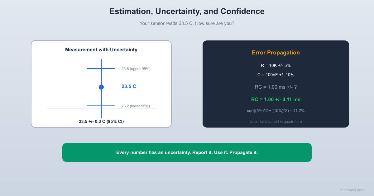
When you combine uncertain quantities in a formula, the uncertainties combine too. If your resistor is kohm (5% tolerance) and your capacitor is nF (10% tolerance), what is the uncertainty in ?
The Simple Rule for Products
For multiplication and division, relative (percentage) uncertainties add in quadrature:
So ms with about 11.2% uncertainty. That means ms.
The following Monte Carlo simulation computes the RC time constant and its uncertainty by sampling component values from their tolerance distributions. It then compares the result to the analytical formula above.
error_propagation_monte_carlo.py
import numpy as np
np.random.seed(42)
n_samples =100000
# Component nominal values and tolerances
R_nom =10e3# 10 kohm
R_tol =0.05# 5%
C_nom =100e-9# 100 nF
C_tol =0.10# 10%
# Monte Carlo: sample from uniform distributions within tolerance bands
print(f" Std: {tau_analytical_std*1e3:.4f} ms (relative = {rel_unc*100:.1f}%)")
print(f"\nThe Monte Carlo and analytical results agree closely.")
print(f"Your 1.0 ms time constant is really 1.0 +/- {tau_std*1e3:.2f} ms.")
The Simple Rule for Sums
For addition and subtraction, absolute uncertainties add in quadrature:
If you measure two voltages V and V, the difference is:
Tolerance Stackup in Practice
This is not abstract theory. In mechanical engineering, if you stack five parts each with mm tolerance, the total stackup is not mm (that is the worst case). The statistical stackup is mm. Knowing the difference between worst-case and statistical stackup can save you money on manufacturing tolerances.
When to Use Worst-Case vs. Statistical Analysis
Situation
Use
Safety-critical systems (medical, automotive, aerospace)
Worst-case analysis
High-volume consumer products where occasional failure is acceptable
Statistical analysis
Low-volume production where every unit must work
Worst-case analysis
Early design phase, rough sizing
Statistical analysis
Final verification before manufacturing release
Both, and compare
The choice between worst-case and statistical analysis is itself an engineering judgment. In general, if the consequence of exceeding the tolerance is catastrophic (a bridge collapses, a pacemaker fails), use worst-case. If the consequence is minor (a slightly loose fit that can be reworked), statistical analysis saves cost.
Uncertainty in Software
Uncertainty is not just for hardware. Software systems have uncertainty too, though it takes different forms:
Latency uncertainty. A network request might take 10 ms or 500 ms. Your system design needs to handle both.
Load uncertainty. You might get 100 requests per second or 10,000. Your capacity planning must account for the range.
Input uncertainty. User inputs might be well-formed or garbage. Your parser needs to handle both gracefully.
Clock uncertainty. System clocks drift. NTP corrections are not instantaneous. Distributed timestamps might disagree.
The same principles apply: estimate the range, propagate through your design, and report your confidence honestly. “The system handles up to 5000 requests per second” is much more useful than “the system is fast.”
Confidence Intervals
When you report a measurement as C, the could mean several things. Is it the standard deviation of your measurements? The range? A 95% confidence interval?
What a 95% Confidence Interval Means
A 95% confidence interval means: if you repeated this measurement many times and computed the interval each time, about 95% of those intervals would contain the true value. It does not mean there is a 95% probability the true value is in this particular interval (a subtle but important distinction that trips up even experienced scientists).
Computing a Confidence Interval
Suppose you measure a voltage 10 times and get these values:
Trial
Voltage (V)
1
3.28
2
3.31
3
3.29
4
3.33
5
3.30
6
3.27
7
3.32
8
3.29
9
3.31
10
3.30
The mean is V. The standard deviation is V. The standard error of the mean is V.
For a 95% confidence interval with 9 degrees of freedom, the t-value is about 2.26. So the 95% CI is:
You would report this as: “The voltage is 3.300 V (95% CI: 3.287 to 3.313 V).”
Measurement Uncertainty Budgets
In professional metrology, you build an uncertainty budget: a table listing every source of uncertainty and its contribution. For a temperature measurement, your budget might look like this:
Source
Type
Uncertainty (C)
Sensor calibration
Systematic
0.10
ADC quantization
Systematic
0.05
Self-heating
Systematic
0.02
Noise (random)
Random
0.08
Combined
0.14
The combined uncertainty is the quadrature sum of all sources: C.
Systematic vs. Random Uncertainty
Notice the “Type” column in the table above. There are two fundamentally different kinds of uncertainty:
Random (Type A)
Random uncertainty varies unpredictably from measurement to measurement. Electrical noise is a classic example. You can reduce random uncertainty by averaging multiple measurements: the standard error decreases as , so 100 measurements give 10x less random uncertainty than a single measurement.
Systematic (Type B)
Systematic uncertainty is consistent and repeatable. A miscalibrated sensor always reads 0.2 C too high. Averaging does not help because every measurement has the same bias. You reduce systematic uncertainty through calibration, better equipment, or correction formulas.
When you see a measurement that looks “stable” (low variation between readings), do not assume it is accurate. It might have low random uncertainty but high systematic uncertainty. The readings are precise (they agree with each other) but not accurate (they are all wrong by the same amount).
Putting It All Together
Here is a practical workflow for handling numbers honestly in engineering:
Estimate first. Before you measure or calculate, do a quick Fermi estimate. This gives you a sanity check.
Know your instrument’s limits. What is the resolution? What is the accuracy? These set a floor on your uncertainty.
Report the right number of significant figures. Match your reporting precision to your measurement precision. No more, no less.
Propagate uncertainty through calculations. If you combine uncertain quantities, the result is uncertain too. Compute it.
State your confidence. When you report a number, say what the uncertainty means. Is it a standard deviation? A 95% confidence interval? A worst-case bound?
The Key Question
The single most important habit you can build as an engineer is asking: “How sure am I about this number?”
Not just “what is the number?” but “what is the range of values it could reasonably be?” If you cannot answer that question, you do not really know the number. You have a guess that looks precise.
Think About It
Next time you read a spec sheet, notice how the manufacturer reports values. A 10 kohm resistor with 1% tolerance is kohm. A 3.3 V regulator with 2% accuracy outputs V. These are not just numbers on a page. They are promises about what the component will actually do in your circuit.
Common Mistakes Engineers Make With Numbers
Even experienced engineers routinely make mistakes with uncertainty and estimation. Here are the most frequent ones, along with how to avoid them.
Treating Typical Values as Guaranteed
Datasheets often list three columns: minimum, typical, and maximum. The typical value is measured on a sample of parts under specific conditions. It is not a guarantee. If your design only works at the typical value and fails at the minimum or maximum, your design is broken.
Design to the Limits
Always design to the minimum and maximum values in the datasheet. The typical value tells you what is common. The min/max values tell you what is possible. Your design must work across the full range, not just at the center.
Ignoring Temperature Effects
Component values drift with temperature. A ceramic capacitor rated at 100 nF might actually be 80 nF at your operating temperature if it uses X5R dielectric. A crystal oscillator rated at 20 MHz might be 20.0004 MHz on a hot day. If your design is temperature-sensitive, check the temperature coefficients in the datasheet and include them in your uncertainty budget.
Confusing Resolution with Accuracy
A 16-bit ADC has 65,536 counts of resolution. That does not mean your measurement is accurate to 1 part in 65,536. The ADC also has offset error, gain error, nonlinearity, and noise, all of which are separate from resolution. A 16-bit ADC with 2 LSB of noise and 5 LSB of offset error effectively gives you about 13 to 14 bits of useful accuracy, not 16.
Specification
What It Means
Resolution
Smallest change you can detect
Accuracy
How close the reading is to the true value
Precision
How repeatable the reading is
Noise
Random variation in the reading
High resolution with poor accuracy is like a ruler with very fine markings that starts at 0.3 instead of 0.0. You can read it to the nearest 0.1 mm, but every reading is off by 0.3 mm.
Forgetting About Units
Unit errors have crashed spacecraft (the Mars Climate Orbiter was lost because one team used metric units and another used imperial). They have caused drug overdoses in hospitals. They are among the most common and most preventable engineering errors.
When you propagate uncertainty through a calculation, carry the units through every step. If the units do not come out right at the end, you made an error somewhere. Units are not just labels; they are a type-checking system for physics.
How Much Effort to Spend on Uncertainty
Not every number deserves a full uncertainty analysis. The key question is: does the uncertainty matter for this decision?
Comparing two options that are close in performance. If MCU A draws 50 uA and MCU B draws 55 uA, you need to know the uncertainty to decide whether the difference is real.
The goal is not to analyze everything to the last decimal place. The goal is to know when precision matters and when it does not, and to act accordingly.
The Cost of Over-Precision
Demanding unnecessary precision costs time and money. If your tolerance analysis says you need a 0.1% resistor but a 1% resistor would work fine, you are paying 5 to 10 times more per resistor for no benefit. If you spend three hours computing a confidence interval for a measurement that only needs to be “roughly 3 V,” you have wasted three hours.
Good engineering judgment means matching the precision of your analysis to the needs of your application. Not more, not less.
Exercises
Fermi estimation. How many lines of code are in the Linux kernel? Start from what you know (it is a large project, started in 1991, has thousands of contributors) and work your way to an order-of-magnitude estimate. Then look up the actual number and see how close you got.
Significant figures. Your 12-bit ADC has a 5.0 V reference. You read a raw value of 2048. How many significant figures should you report in the computed voltage? What is the honest voltage value?
Error propagation. You are designing a voltage divider with kohm and kohm. The output voltage is . If V, what is and its uncertainty?
Confidence intervals. You measure the response time of a web server 20 times and get a mean of 142 ms with a standard deviation of 18 ms. Compute the 95% confidence interval for the mean response time. (Hint: the t-value for 19 degrees of freedom at 95% is about 2.09.)
Summary
Every engineering number carries uncertainty, and ignoring that uncertainty leads to false confidence in your designs. Fermi estimation gives you fast sanity checks. Significant figures prevent you from claiming precision you do not have. Error propagation tells you how uncertainties combine. Confidence intervals let you state precisely how sure you are. The habit of asking “how sure am I?” about every number is one of the most valuable thinking tools an engineer can develop.
Comments