Four-Bar Linkage Experiments
Every mechanism textbook presents the Grashof condition as a simple inequality: s + l must be less than or equal to p + q. Students memorize it, apply it on exams, and move on. But what does it actually look like when a mechanism transitions from Grashof to non-Grashof? What happens to the transmission angle, the velocity ratios, the coupler curve? These experiments let you see, measure, and analyze the behaviors that the inequality alone cannot convey. #FourBarLinkage #GrashofCondition #MechanismDesign
Key Terms
| Term | Meaning |
|---|---|
| a | Input crank length (mm), the driven link |
| b | Coupler length (mm), the floating link connecting the two moving joints |
| c | Follower/rocker length (mm), the output link |
| d | Ground/frame length (mm), the fixed distance between the two pivot points |
| Grashof | A linkage where s + l is at most p + q (s = shortest, l = longest, p and q = remaining). At least one link can make a full rotation |
| Crank-rocker | Grashof linkage where the shortest link is the input: it rotates fully while the output oscillates |
| Double-crank | Grashof linkage where the shortest link is the ground: both input and output rotate fully |
| Double-rocker | Either non-Grashof (no full rotation) or Grashof with the coupler as shortest link |
| Transmission angle | The angle between the coupler and follower. Below about 40 degrees, force transmission becomes poor |
| Coupler curve | The path traced by a point on the coupler link as the mechanism moves |
| Circuit | The two possible assembly configurations (open and crossed) for the same link lengths |
Experiment Workflow
Setting Up Your Workspace
Directoryfour-bar-lab/
Directorydata/
- exp1_grashof.csv
- exp2_transmission.csv
- exp3_presets.csv
- exp4_circuits.csv
- exp5_coupler.csv
- exp6_sensitivity.csv
- exp9_offset.csv
Directoryplots/
- …
Directoryscripts/
- experiment_1_grashof.py
- experiment_2_transmission.py
- experiment_3_presets.py
- experiment_6_sensitivity.py
- experiment_9_ground_offset.py
How to Record Data
For each experiment, read values from the simulator’s charts and summary panels. Save as CSV files. Alternatively, download the complete CSV from the simulator’s download section.
Experiment 1: The Grashof Condition
Every four-bar linkage falls into one of two categories: Grashof (at least one link can fully rotate) or non-Grashof (no link can complete a full turn). This single classification determines whether a mechanism can be used as a crank input or only as a rocker. The Grashof inequality is simple math, but watching a mechanism transition from rotatable to locked is something no equation can convey. You will build four configurations, predict their classification, and verify against the simulator.
-
Crank-rocker (Grashof) Set a=40, b=120, c=80, d=100. Predict: s+l = 40+120 = 160, p+q = 80+100 = 180. Grashof: yes. Run the experiment and start the animation. The input crank should complete full rotations.
-
Make it non-Grashof Change a=80 (so now s=80, l=120, s+l=200 is greater than p+q=180). Run the experiment. The animation should stop at certain angles because the crank cannot complete a full rotation.
-
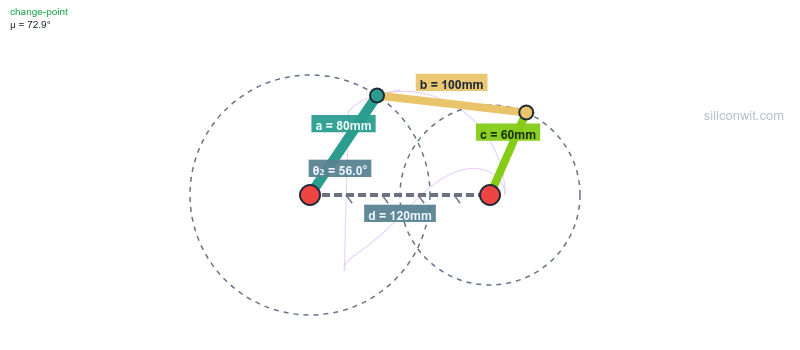
Boundary case Set a=60, b=120, c=80, d=100. Now s+l = 60+120 = 180 = p+q. This is a change-point mechanism. Run and observe the behavior at the singular positions.
-
Record Grashof status For each configuration, note whether the crank completes a full rotation, the Grashof type shown in the simulator, and the minimum transmission angle. Save as
data/exp1_grashof.csv.
Data Collection Table
| Configuration | s+l | p+q | Grashof? | Full rotation? | Min transmission angle |
|---|---|---|---|---|---|
| a=40, b=120, c=80, d=100 | |||||
| a=80, b=120, c=80, d=100 | |||||
| a=60, b=120, c=80, d=100 | |||||
| a=20, b=80, c=60, d=50 |
Python Analysis
import numpy as npimport matplotlib.pyplot as pltimport csvimport os
# ============================================================# STEP 1: Load your CSV data from the simulator# Place your downloaded CSV in the data/ folder, or update the path# ============================================================csv_file = 'data/exp1_baseline.csv'sim_data = None
if os.path.exists(csv_file):    with open(csv_file) as f:        reader = csv.DictReader(f)        sim_data = list(reader)    print(f"Loaded {len(sim_data)} rows from {csv_file}")else:    print(f"No CSV found at {csv_file}. Using analytical data only.")    print("To use simulator data: download CSV from the simulator or")    print("record values from the charts into a CSV with these columns:")    print("Input Angle (deg), Coupler Angle (deg), Follower Angle (deg), ...")
# ============================================================# STEP 2: Analytical computation (for comparison)# ============================================================def solve_fourbar(a, b, c, d, e, theta2_deg):    t2 = np.radians(theta2_deg)    Ax, Ay = a*np.cos(t2), a*np.sin(t2)    dx, dy = d - Ax, e - Ay    dist = np.sqrt(dx**2 + dy**2)    if dist > b+c or dist < abs(b-c) or dist < 1e-10:        return None    ca = (b**2 - c**2 + dist**2) / (2*dist)    hsq = b**2 - ca**2    if hsq < 0: return None    h = np.sqrt(hsq)    mx, my = Ax + ca*dx/dist, Ay + ca*dy/dist    Bx, By = mx + h*dy/dist, my - h*dx/dist    t3 = np.degrees(np.arctan2(By-Ay, Bx-Ax))    t4 = np.degrees(np.arctan2(By-e, Bx-d))    return {'theta3': t3, 'theta4': t4}
# Test Grashof condition for multiple configurationsconfigs = [    {'a': 40, 'b': 120, 'c': 80, 'd': 100, 'e': 0, 'name': 'Crank-rocker'},    {'a': 80, 'b': 120, 'c': 80, 'd': 100, 'e': 0, 'name': 'Non-Grashof'},    {'a': 60, 'b': 120, 'c': 80, 'd': 100, 'e': 0, 'name': 'Change-point'},    {'a': 60, 'b': 80, 'c': 70, 'd': 40, 'e': 0, 'name': 'Double-crank'},]
print("\nGrashof Classification:")for cfg in configs:    D = np.sqrt(cfg['d']**2 + cfg['e']**2)    links = sorted([cfg['a'], cfg['b'], cfg['c'], D])    s, l = links[0], links[3]    grashof = 'Grashof' if s + l <= links[1] + links[2] else 'Non-Grashof'    if abs(s + l - links[1] - links[2]) < 0.01: grashof = 'Change-point'    valid = sum(1 for t in range(361) if solve_fourbar(cfg['a'],cfg['b'],cfg['c'],cfg['d'],cfg['e'],t))    print(f"  {cfg['name']}: s+l={s+l:.0f}, p+q={links[1]+links[2]:.0f} -> {grashof}, valid={valid}/361")
# ============================================================# STEP 3: If CSV loaded, plot simulator data vs analytical# ============================================================if sim_data:    sim_angles = [float(r['Input Angle (deg)']) for r in sim_data]    sim_theta3 = [float(r['Coupler Angle (deg)']) for r in sim_data]    sim_theta4 = [float(r['Follower Angle (deg)']) for r in sim_data]
    # Compute analytical for baseline config    a, b, c, d, e = 40, 120, 80, 100, 0    anal_theta3, anal_theta4 = [], []    for t in sim_angles:        r = solve_fourbar(a, b, c, d, e, t)        anal_theta3.append(r['theta3'] if r else np.nan)        anal_theta4.append(r['theta4'] if r else np.nan)
    fig, axes = plt.subplots(2, 1, figsize=(10, 8), sharex=True)    axes[0].plot(sim_angles, sim_theta3, 'b-', label='Simulator', linewidth=2)    axes[0].plot(sim_angles, anal_theta3, 'r--', label='Analytical', linewidth=1)    axes[0].set_ylabel('Coupler Angle (deg)')    axes[0].legend()    axes[0].set_title('Experiment 1: Simulator vs Analytical Comparison')
    axes[1].plot(sim_angles, sim_theta4, 'b-', label='Simulator', linewidth=2)    axes[1].plot(sim_angles, anal_theta4, 'r--', label='Analytical', linewidth=1)    axes[1].set_ylabel('Follower Angle (deg)')    axes[1].set_xlabel('Input Angle (deg)')    axes[1].legend()
    plt.tight_layout()    plt.savefig('plots/experiment_1_comparison.png', dpi=150)    plt.show()
    # Compute error    errors = [abs(s - a) for s, a in zip(sim_theta4, anal_theta4) if not np.isnan(a)]    print(f"\nFollower angle: max error = {max(errors):.4f} deg, mean error = {np.mean(errors):.4f} deg")
Expected Results
- a=40, b=120, c=80, d=100: Grashof (s+l=160 < p+q=180), crank completes full rotation
- a=80, b=120, c=80, d=100: Non-Grashof (s+l=200 > p+q=180), crank locks at certain angles
- a=60, b=120, c=80, d=100: Change-point (s+l=180 = p+q), mechanism reaches singular positions
- a=20, b=80, c=60, d=50: Grashof double-crank (shortest link is ground)
Design Question
You need a mechanism where the input crank makes full rotations but the output oscillates. Which link must be the shortest? What happens if manufacturing errors make one link 2mm longer than specified, pushing s+l past the boundary?
Challenge: Ground Offset Preview
Try increasing the ground offset slider from 0 to 50mm on the crank-rocker preset. Watch the Grashof indicator change. At what offset does the mechanism lose its crank-rocker behavior? This is explored in full detail in Experiment 9.
Experiment 2: Transmission Angle and Mechanism Quality
A mechanism can satisfy the Grashof condition and still be useless if the transmission angle drops too low. The transmission angle determines how effectively force is transmitted from input to output. Below about 40 degrees, friction and compliance dominate, and the mechanism feels “dead.” This experiment quantifies where the transmission angle problems occur and how link proportions control them.
-
Good transmission angle Use the crank-rocker preset (a=40, b=120, c=80, d=100). Run the experiment. Note the min and max transmission angle from the summary panel.
-
Save as Experiment A
-
Degrade the transmission angle Change c=40 (shorter follower). Run the experiment. The transmission angle should dip lower.
-
Improve the transmission angle Clear Experiment A. Set a=30, b=100, c=90, d=100. Run the experiment. Compare the transmission angle range.
-
Collect data For each configuration, record min and max transmission angle. Save as
data/exp2_transmission.csv. Alternatively, download the CSV from the simulator.
Data Collection Table
| Configuration | Min transmission angle | Max transmission angle | Below 40 degrees? |
|---|---|---|---|
| a=40, b=120, c=80, d=100 | |||
| a=40, b=120, c=40, d=100 | |||
| a=30, b=100, c=90, d=100 |
Python Analysis
import numpy as npimport matplotlib.pyplot as pltimport csvimport os
# ============================================================# STEP 1: Load CSV data from the simulator# Download CSV from the simulator or record from charts# ============================================================csv_files = {    'Baseline': 'data/exp2_baseline.csv',    'Short follower': 'data/exp2_short_follower.csv',    'Improved': 'data/exp2_improved.csv',}sim_datasets = {}for label, path in csv_files.items():    if os.path.exists(path):        with open(path) as f:            sim_datasets[label] = list(csv.DictReader(f))        print(f"Loaded {len(sim_datasets[label])} rows from {path}")    else:        print(f"No CSV at {path} (will use analytical only for {label})")
# ============================================================# STEP 2: Analytical computation (two-circle intersection)# ============================================================def solve_fourbar(a, b, c, d, e, theta2_deg):    t2 = np.radians(theta2_deg)    Ax, Ay = a*np.cos(t2), a*np.sin(t2)    dx, dy = d - Ax, e - Ay    dist = np.sqrt(dx**2 + dy**2)    if dist > b+c or dist < abs(b-c) or dist < 1e-10:        return None    ca = (b**2 - c**2 + dist**2) / (2*dist)    hsq = b**2 - ca**2    if hsq < 0: return None    h = np.sqrt(hsq)    mx, my = Ax + ca*dx/dist, Ay + ca*dy/dist    Bx, By = mx + h*dy/dist, my - h*dx/dist    t3 = np.degrees(np.arctan2(By-Ay, Bx-Ax))    t4 = np.degrees(np.arctan2(By-e, Bx-d))    mu = abs(t3 - t4)    if mu > 180: mu = 360 - mu    if mu > 90: mu = 180 - mu    return {'theta3': t3, 'theta4': t4, 'mu': mu}
configs = [    {'a': 40, 'b': 120, 'c': 80, 'd': 100, 'e': 0, 'label': 'Baseline'},    {'a': 40, 'b': 120, 'c': 40, 'd': 100, 'e': 0, 'label': 'Short follower'},    {'a': 30, 'b': 100, 'c': 90, 'd': 100, 'e': 0, 'label': 'Improved'},]
theta2 = np.arange(0, 361)fig, ax = plt.subplots(figsize=(10, 5))
# ============================================================# STEP 3: Plot simulator data vs analytical# ============================================================for cfg in configs:    # Analytical    mu_anal = []    for t in theta2:        r = solve_fourbar(cfg['a'], cfg['b'], cfg['c'], cfg['d'], cfg['e'], t)        mu_anal.append(r['mu'] if r else np.nan)    mu_anal = np.array(mu_anal)
    label = cfg['label']    if label in sim_datasets:        sim = sim_datasets[label]        sim_angles = [float(row['Input Angle (deg)']) for row in sim]        sim_mu = [float(row['Transmission Angle (deg)']) for row in sim]        ax.plot(sim_angles, sim_mu, '-', label=f'{label} (simulator)', linewidth=2)        ax.plot(theta2, mu_anal, '--', label=f'{label} (analytical)', linewidth=1, alpha=0.7)        # Error        common = min(len(sim_mu), len(mu_anal))        errors = [abs(s - a) for s, a in zip(sim_mu[:common], mu_anal[:common]) if not np.isnan(a)]        if errors:            print(f"{label}: max error = {max(errors):.4f} deg, mean = {np.mean(errors):.4f} deg")    else:        ax.plot(theta2, mu_anal, '-', label=label, linewidth=2)
    valid = mu_anal[~np.isnan(mu_anal)]    print(f"{label}: min mu = {np.nanmin(mu_anal):.1f}, max mu = {np.nanmax(mu_anal):.1f}")
ax.axhline(y=40, color='r', linestyle='--', alpha=0.5, label='40 deg limit')ax.set_xlabel('Input Angle (degrees)')ax.set_ylabel('Transmission Angle (degrees)')ax.set_title('Experiment 2: Transmission Angle Comparison')ax.legend(fontsize=8)plt.tight_layout()plt.savefig('plots/experiment_2_transmission.png', dpi=150)plt.show()
Expected Results
- Baseline (a=40, b=120, c=80, d=100): transmission angle stays well above 40 degrees
- Short follower (c=40): transmission angle dips significantly, potentially below the 40-degree limit
- Improved (a=30, b=100, c=90, d=100): more uniform transmission angle through the cycle
Design Question
You are designing a mechanism for a packaging machine that must transmit force reliably at all positions. What minimum transmission angle would you require? How would you adjust link lengths to achieve it?
Challenge: Quick-Return Time Ratio
For a crank-rocker, the follower spends more time on one stroke than the other (the crank sweeps different arc lengths for forward vs return). Using the time domain toggle (switch x-axis to Time), measure how long the follower takes for the forward swing vs the return swing with the crank-rocker preset. Then add a ground offset of e=30mm. Does the time ratio change? This ratio matters for machines like shapers that need a fast idle return.
Experiment 3: Comparing the Four Presets
A crank-rocker, a double-crank, a double-rocker, and a parallelogram are all four-bar linkages. But they behave completely differently. By overlaying their angular velocity profiles, you can see why each type is suited to different applications: crank-rockers for oscillating output, double-cranks for speed ratio control, parallelograms for parallel motion (like bus doors and drafting machines).
-
Crank-rocker preset Select the preset. Run the experiment. Save as Experiment A.
-
Double-crank preset Select it. Run the experiment. Compare the overlay.
-
Double-rocker and parallelogram Repeat for each, comparing against Experiment A.
-
Collect data For each preset, record: follower oscillation range (theta4 max minus min), max omega4, and min transmission angle. Save as
data/exp3_presets.csv. Alternatively, download the CSV from the simulator for each preset.
Data Collection Table
| Preset | Follower oscillation (degrees) | Max omega4 (rad/s) | Min transmission angle |
|---|---|---|---|
| Crank-Rocker | |||
| Double-Crank | |||
| Double-Rocker | |||
| Parallelogram |
Python Analysis
import numpy as npimport matplotlib.pyplot as pltimport csvimport os
# ============================================================# STEP 1: Load CSV data from the simulator for each preset# Download CSV from the simulator for each preset configuration# ============================================================csv_files = {    'Crank-Rocker': 'data/exp3_crank_rocker.csv',    'Double-Crank': 'data/exp3_double_crank.csv',    'Double-Rocker': 'data/exp3_double_rocker.csv',    'Parallelogram': 'data/exp3_parallelogram.csv',}sim_datasets = {}for name, path in csv_files.items():    if os.path.exists(path):        with open(path) as f:            sim_datasets[name] = list(csv.DictReader(f))        print(f"Loaded {len(sim_datasets[name])} rows for {name}")    else:        print(f"No CSV at {path} (analytical only for {name})")
# ============================================================# STEP 2: Analytical computation (two-circle intersection)# ============================================================def solve_fourbar(a, b, c, d, e, theta2_deg):    t2 = np.radians(theta2_deg)    Ax, Ay = a*np.cos(t2), a*np.sin(t2)    dx, dy = d - Ax, e - Ay    dist = np.sqrt(dx**2 + dy**2)    if dist > b+c or dist < abs(b-c) or dist < 1e-10:        return None    ca = (b**2 - c**2 + dist**2) / (2*dist)    hsq = b**2 - ca**2    if hsq < 0: return None    h = np.sqrt(hsq)    mx, my = Ax + ca*dx/dist, Ay + ca*dy/dist    Bx, By = mx + h*dy/dist, my - h*dx/dist    t3 = np.degrees(np.arctan2(By-Ay, Bx-Ax))    t4 = np.degrees(np.arctan2(By-e, Bx-d))    return {'theta3': t3, 'theta4': t4}
presets = [    {'name': 'Crank-Rocker', 'a': 40, 'b': 120, 'c': 80, 'd': 100, 'e': 0},    {'name': 'Double-Crank', 'a': 60, 'b': 80, 'c': 70, 'd': 40, 'e': 0},    {'name': 'Double-Rocker', 'a': 80, 'b': 35, 'c': 60, 'd': 100, 'e': 0},    {'name': 'Parallelogram', 'a': 60, 'b': 100, 'c': 60, 'd': 100, 'e': 0},]
theta2 = np.arange(0, 361)
# ============================================================# STEP 3: Plot simulator data vs analytical for each preset# ============================================================fig, axes = plt.subplots(2, 1, figsize=(10, 8), sharex=True)colors = ['blue', 'red', 'green', 'orange']
for idx, p in enumerate(presets):    # Analytical    t4_anal = []    for t in theta2:        r = solve_fourbar(p['a'], p['b'], p['c'], p['d'], p['e'], t)        t4_anal.append(r['theta4'] if r else np.nan)    t4_anal = np.array(t4_anal)
    name = p['name']    if name in sim_datasets:        sim = sim_datasets[name]        sim_angles = [float(row['Input Angle (deg)']) for row in sim]        sim_t4 = [float(row['Follower Angle (deg)']) for row in sim]        sim_omega4 = [float(row['Omega4 (rad/s)']) for row in sim]        axes[0].plot(sim_angles, sim_t4, '-', color=colors[idx],                     label=f'{name} (sim)', linewidth=2)        axes[0].plot(theta2, t4_anal, '--', color=colors[idx],                     label=f'{name} (anal)', linewidth=1, alpha=0.6)        axes[1].plot(sim_angles, sim_omega4, '-', color=colors[idx],                     label=f'{name}', linewidth=2)    else:        axes[0].plot(theta2, t4_anal, '-', color=colors[idx],                     label=name, linewidth=2)
    valid = t4_anal[~np.isnan(t4_anal)]    if len(valid) > 0:        osc = np.nanmax(t4_anal) - np.nanmin(t4_anal)        print(f"{name}: theta4 = {np.nanmin(t4_anal):.1f} to {np.nanmax(t4_anal):.1f} ({osc:.1f} deg)")
axes[0].set_ylabel('Follower Angle theta4 (deg)')axes[0].set_title('Experiment 3: Four-Bar Presets Comparison')axes[0].legend(fontsize=8)axes[1].set_ylabel('Follower Omega4 (rad/s)')axes[1].set_xlabel('Input Angle theta2 (deg)')axes[1].legend(fontsize=8)
plt.tight_layout()plt.savefig('plots/experiment_3_presets.png', dpi=150)plt.show()
Expected Results
- Crank-rocker: follower oscillates over a limited range (typically 40-80 degrees)
- Double-crank: both links rotate fully, follower angle covers 360 degrees
- Double-rocker: neither input nor output completes full rotation, both oscillate
- Parallelogram: follower angle tracks input angle exactly (constant velocity ratio of 1)
Analysis Question
A windshield wiper needs oscillating output from a rotating motor. Which preset matches this requirement? A conveyor belt needs both sprockets to rotate continuously. Which preset fits? What makes the parallelogram special for applications like bus doors and drafting machines?
Challenge: Find Your Own Application
Identify a real mechanism around you (a door closer, a folding chair, a car hood hinge, a pair of pliers, a bicycle brake lever) and try to estimate its link lengths. Enter them in the simulator and see if the behavior matches what you observe in real life. Document: what type of four-bar is it? Does it match a Grashof classification? What is its transmission angle range?
Experiment 4: Open vs Crossed Circuit
Every four-bar linkage has two valid assembly configurations for the same link lengths: open and crossed. Most textbooks mention this in passing, but the difference is dramatic. The same physical links produce completely different motion, different transmission angles, and different velocity profiles depending on which circuit you use. The simulator lets you switch between them instantly.
-
Open circuit Use crank-rocker preset (a=40, b=120, c=80, d=100). Ensure circuit is “Open”. Run the experiment. Save as Experiment A.
-
Crossed circuit Change the assembly configuration to “Crossed”. Run the experiment. Compare the overlay, especially the transmission angle.
-
Collect data Record theta4 range and min transmission angle for each circuit. Save as
data/exp4_circuits.csv. Alternatively, download the CSV from the simulator for each configuration.
Data Collection Table
| Circuit | θ₄ min | θ₄ max | Oscillation | Min μ |
|---|---|---|---|---|
| Open | ||||
| Crossed |
Design Question
In what situations would an engineer deliberately choose the crossed circuit over the open circuit?
Python Analysis
import numpy as npimport matplotlib.pyplot as pltimport csvimport os
# ============================================================# STEP 1: Load CSV data from the simulator# Run the simulator in Open circuit, download CSV# Then switch to Crossed circuit, download CSV# ============================================================csv_files = {    'Open': 'data/exp4_open.csv',    'Crossed': 'data/exp4_crossed.csv',}sim_datasets = {}for label, path in csv_files.items():    if os.path.exists(path):        with open(path) as f:            sim_datasets[label] = list(csv.DictReader(f))        print(f"Loaded {len(sim_datasets[label])} rows for {label}")    else:        print(f"No CSV at {path} (analytical only for {label})")
# ============================================================# STEP 2: Analytical computation (two-circle intersection)# Open circuit: B above the line A-O4# Crossed circuit: B below the line A-O4# ============================================================def solve_fourbar_circuit(a, b, c, d, e, theta2_deg, circuit='open'):    t2 = np.radians(theta2_deg)    Ax, Ay = a*np.cos(t2), a*np.sin(t2)    dx, dy = d - Ax, e - Ay    dist = np.sqrt(dx**2 + dy**2)    if dist > b+c or dist < abs(b-c) or dist < 1e-10:        return None    ca = (b**2 - c**2 + dist**2) / (2*dist)    hsq = b**2 - ca**2    if hsq < 0: return None    h = np.sqrt(hsq)    mx, my = Ax + ca*dx/dist, Ay + ca*dy/dist    sign = 1 if circuit == 'open' else -1    Bx = mx + sign * h * dy / dist    By = my - sign * h * dx / dist    t4 = np.degrees(np.arctan2(By - e, Bx - d))    t3 = np.degrees(np.arctan2(By - Ay, Bx - Ax))    mu = abs(t3 - t4)    if mu > 180: mu = 360 - mu    if mu > 90: mu = 180 - mu    return {'theta4': t4, 'mu': mu}
a, b, c, d, e = 40, 120, 80, 100, 0theta2 = np.arange(0, 361)
# ============================================================# STEP 3: Plot simulator data vs analytical# ============================================================fig, axes = plt.subplots(2, 1, figsize=(10, 8), sharex=True)circuit_colors = {'Open': 'blue', 'Crossed': 'red'}
for circuit in ['Open', 'Crossed']:    # Analytical    t4_anal, mu_anal = [], []    for t in theta2:        r = solve_fourbar_circuit(a, b, c, d, e, t, circuit.lower())        t4_anal.append(r['theta4'] if r else np.nan)        mu_anal.append(r['mu'] if r else np.nan)    t4_anal = np.array(t4_anal)    mu_anal = np.array(mu_anal)    color = circuit_colors[circuit]
    if circuit in sim_datasets:        sim = sim_datasets[circuit]        sim_angles = [float(row['Input Angle (deg)']) for row in sim]        sim_t4 = [float(row['Follower Angle (deg)']) for row in sim]        sim_mu = [float(row['Transmission Angle (deg)']) for row in sim]        axes[0].plot(sim_angles, sim_t4, '-', color=color,                     label=f'{circuit} (simulator)', linewidth=2)        axes[0].plot(theta2, t4_anal, '--', color=color,                     label=f'{circuit} (analytical)', linewidth=1, alpha=0.6)        axes[1].plot(sim_angles, sim_mu, '-', color=color, label=f'{circuit} (sim)', linewidth=2)        axes[1].plot(theta2, mu_anal, '--', color=color, label=f'{circuit} (anal)', linewidth=1, alpha=0.6)    else:        axes[0].plot(theta2, t4_anal, '-', color=color, label=circuit, linewidth=2)        axes[1].plot(theta2, mu_anal, '-', color=color, label=circuit, linewidth=2)
    valid = t4_anal[~np.isnan(t4_anal)]    if len(valid) > 0:        print(f"{circuit}: theta4 = {np.nanmin(t4_anal):.1f} to {np.nanmax(t4_anal):.1f}")        print(f"{circuit}: min mu = {np.nanmin(mu_anal):.1f}, max mu = {np.nanmax(mu_anal):.1f}")
axes[0].set_ylabel('Follower Angle (deg)')axes[0].set_title('Experiment 4: Open vs Crossed Circuit')axes[0].legend(fontsize=8)axes[1].set_ylabel('Transmission Angle (deg)')axes[1].set_xlabel('Input Angle (deg)')axes[1].axhline(y=40, color='gray', linestyle='--', alpha=0.5, label='40 deg limit')axes[1].legend(fontsize=8)
plt.tight_layout()plt.savefig('plots/experiment_4_circuits.png', dpi=150)plt.show()
Expected Results
- The open and crossed circuits produce completely different theta4 profiles for the same link lengths
- One circuit typically has better transmission angle than the other
- The crossed circuit may have the follower rotating in the opposite sense
Experiment 5: Coupler Curve Exploration
The coupler curve is perhaps the most powerful and least appreciated feature of the four-bar linkage. The path traced by a point on the coupler can approximate straight lines, circles, figure-eights, and complex shapes depending on the link proportions and point location. This is how mechanisms generate complex output motion from simple rotary input, without gears or cams.
-
Crank-rocker coupler curve Use the crank-rocker preset. Enable “Show Paths and Coupler Curve”. The purple trace shows the coupler midpoint path.
-
Change link proportions Try a=30, b=150, c=100, d=100. The coupler curve changes dramatically.
-
Parallelogram Use the parallelogram preset. The coupler curve should be a circle (all points on the coupler trace circles when a=c and b=d).
-
Observe and sketch For each configuration, observe the coupler curve shape and note whether any portion approximates a straight line.
-
Collect data For each configuration, note the coupler curve shape (circle, ellipse, figure-eight, kidney, or other) and whether any segment is approximately straight. Save observations as
data/exp5_coupler.csv.
Python Analysis
import numpy as npimport matplotlib.pyplot as pltimport csvimport os
# ============================================================# STEP 1: Load CSV data from the simulator# The CSV includes Ax, Ay, Bx, By columns for coupler midpoint# ============================================================csv_files = {    'Crank-Rocker': 'data/exp5_crank_rocker.csv',    'Long coupler': 'data/exp5_long_coupler.csv',    'Parallelogram': 'data/exp5_parallelogram.csv',}sim_datasets = {}for name, path in csv_files.items():    if os.path.exists(path):        with open(path) as f:            sim_datasets[name] = list(csv.DictReader(f))        print(f"Loaded {len(sim_datasets[name])} rows for {name}")    else:        print(f"No CSV at {path} (analytical only for {name})")
# ============================================================# STEP 2: Analytical computation (two-circle intersection)# ============================================================def solve_fourbar(a, b, c, d, e, theta2_deg):    t2 = np.radians(theta2_deg)    Ax, Ay = a*np.cos(t2), a*np.sin(t2)    dx, dy = d - Ax, e - Ay    dist = np.sqrt(dx**2 + dy**2)    if dist > b+c or dist < abs(b-c) or dist < 1e-10:        return None    ca_val = (b**2 - c**2 + dist**2) / (2*dist)    hsq = b**2 - ca_val**2    if hsq < 0: return None    h = np.sqrt(hsq)    mx, my = Ax + ca_val*dx/dist, Ay + ca_val*dy/dist    Bx, By = mx + h*dy/dist, my - h*dx/dist    return {'Ax': Ax, 'Ay': Ay, 'Bx': Bx, 'By': By}
configs = [    {'a': 40, 'b': 120, 'c': 80, 'd': 100, 'e': 0, 'name': 'Crank-Rocker'},    {'a': 30, 'b': 150, 'c': 100, 'd': 100, 'e': 0, 'name': 'Long coupler'},    {'a': 60, 'b': 100, 'c': 60, 'd': 100, 'e': 0, 'name': 'Parallelogram'},]
theta2 = np.arange(0, 361)
# ============================================================# STEP 3: Plot simulator coupler curves vs analytical# ============================================================fig, axes = plt.subplots(1, 3, figsize=(14, 5))
for idx, cfg in enumerate(configs):    name = cfg['name']
    # Analytical coupler midpoint    mx_a, my_a = [], []    for t in theta2:        r = solve_fourbar(cfg['a'], cfg['b'], cfg['c'], cfg['d'], cfg['e'], t)        if r is None: continue        mx_a.append((r['Ax'] + r['Bx']) / 2)        my_a.append((r['Ay'] + r['By']) / 2)
    if name in sim_datasets:        sim = sim_datasets[name]        # Compute coupler midpoint from simulator joint coordinates        sim_mx = [(float(row['Ax (mm)']) + float(row['Bx (mm)'])) / 2 for row in sim]        sim_my = [(float(row['Ay (mm)']) + float(row['By (mm)'])) / 2 for row in sim]        axes[idx].plot(sim_mx, sim_my, 'b-', label='Simulator', linewidth=2)        axes[idx].plot(mx_a, my_a, 'r--', label='Analytical', linewidth=1)        axes[idx].legend(fontsize=8)    else:        axes[idx].plot(mx_a, my_a, 'purple', linewidth=2)
    axes[idx].set_aspect('equal')    axes[idx].set_title(name)    axes[idx].set_xlabel('X (mm)')    axes[idx].set_ylabel('Y (mm)')    axes[idx].grid(True, alpha=0.3)
plt.suptitle('Experiment 5: Coupler Midpoint Curves')plt.tight_layout()plt.savefig('plots/experiment_5_coupler.png', dpi=150)plt.show()
Expected Results
- Crank-rocker: oval or kidney-shaped coupler curve
- Long coupler: more elongated curve, potentially with a near-straight segment
- Parallelogram: perfect circle (because the coupler translates without rotating)
Design Question
A packaging machine needs a mechanism that moves a part in an approximately straight line over a 50mm segment. Could you achieve this with a four-bar linkage? Which link proportions would you try, and how would you verify straightness from the coupler curve?
Experiment 6: Parametric Sensitivity
When designing a four-bar linkage, you need to know which dimensions matter most. If manufacturing tolerance on the ground link is tight but the coupler can vary, do you care? This experiment quantifies how sensitive the follower oscillation range and minimum transmission angle are to each link length, giving you the data to set rational tolerances.
-
Baseline Set a=40, b=120, c=80, d=100. Record follower oscillation and min transmission angle.
-
Vary input crank (a) Change a to 30, 40, 50, 60 mm (keep b=120, c=80, d=100). Record for each.
-
Vary coupler (b) Reset a=40. Change b to 100, 110, 120, 130, 140 mm. Record for each.
-
Vary ground (d) Reset b=120. Change d to 80, 90, 100, 110, 120 mm. Record for each.
-
Collect data Save all measurements as
data/exp6_sensitivity.csv. Alternatively, download the CSV from the simulator for each configuration.
Python Analysis
import numpy as npimport matplotlib.pyplot as pltimport csvimport os
# ============================================================# STEP 1: Load CSV data from the simulator# Run the simulator for each parameter variation, download CSV# Name files: exp6_a30.csv, exp6_a40.csv, exp6_b100.csv, etc.# ============================================================csv_dir = 'data'sim_data_a, sim_data_b, sim_data_d = {}, {}, {}
for a_val in [30, 35, 40, 45, 50, 55, 60]:    path = os.path.join(csv_dir, f'exp6_a{a_val}.csv')    if os.path.exists(path):        with open(path) as f:            rows = list(csv.DictReader(f))        t4 = [float(r['Follower Angle (deg)']) for r in rows if float(r['Follower Angle (deg)']) != 0]        if t4:            sim_data_a[a_val] = max(t4) - min(t4)
for b_val in [100, 110, 120, 130, 140]:    path = os.path.join(csv_dir, f'exp6_b{b_val}.csv')    if os.path.exists(path):        with open(path) as f:            rows = list(csv.DictReader(f))        t4 = [float(r['Follower Angle (deg)']) for r in rows if float(r['Follower Angle (deg)']) != 0]        if t4:            sim_data_b[b_val] = max(t4) - min(t4)
for d_val in [80, 90, 100, 110, 120]:    path = os.path.join(csv_dir, f'exp6_d{d_val}.csv')    if os.path.exists(path):        with open(path) as f:            rows = list(csv.DictReader(f))        t4 = [float(r['Follower Angle (deg)']) for r in rows if float(r['Follower Angle (deg)']) != 0]        if t4:            sim_data_d[d_val] = max(t4) - min(t4)
loaded = len(sim_data_a) + len(sim_data_b) + len(sim_data_d)print(f"Loaded simulator data for {loaded} configurations")if loaded == 0:    print("No CSV files found. Using analytical data only.")    print("Download CSVs from the simulator for each parameter variation.")
# ============================================================# STEP 2: Analytical computation (two-circle intersection)# ============================================================def get_oscillation(a, b, c, d, e=0):    t4_arr = []    for t in range(361):        t2 = np.radians(t)        Ax, Ay = a*np.cos(t2), a*np.sin(t2)        dx, dy = d - Ax, e - Ay        dist = np.sqrt(dx**2 + dy**2)        if dist > b+c or dist < abs(b-c) or dist < 1e-10:            continue        ca = (b**2 - c**2 + dist**2) / (2*dist)        hsq = b**2 - ca**2        if hsq < 0: continue        h = np.sqrt(hsq)        mx, my = Ax + ca*dx/dist, Ay + ca*dy/dist        Bx, By = mx + h*dy/dist, my - h*dx/dist        t4_arr.append(np.degrees(np.arctan2(By-e, Bx-d)))    if len(t4_arr) < 10: return None    return max(t4_arr) - min(t4_arr)
# ============================================================# STEP 3: Plot simulator data vs analytical# ============================================================fig, axes = plt.subplots(1, 3, figsize=(14, 4))
# Vary aa_vals = np.arange(25, 65, 5)osc_a = [get_oscillation(a, 120, 80, 100) for a in a_vals]axes[0].plot(a_vals, osc_a, 'b-', label='Analytical', linewidth=2)if sim_data_a:    sa_x = sorted(sim_data_a.keys())    axes[0].plot(sa_x, [sim_data_a[k] for k in sa_x], 'ro', label='Simulator', markersize=8)    axes[0].legend(fontsize=8)axes[0].set_xlabel('Crank Length a (mm)')axes[0].set_ylabel('Follower Oscillation (deg)')axes[0].set_title('Sensitivity to a')
# Vary bb_vals = np.arange(100, 145, 5)osc_b = [get_oscillation(40, b, 80, 100) for b in b_vals]axes[1].plot(b_vals, osc_b, 'r-', label='Analytical', linewidth=2)if sim_data_b:    sb_x = sorted(sim_data_b.keys())    axes[1].plot(sb_x, [sim_data_b[k] for k in sb_x], 'bo', label='Simulator', markersize=8)    axes[1].legend(fontsize=8)axes[1].set_xlabel('Coupler Length b (mm)')axes[1].set_title('Sensitivity to b')
# Vary dd_vals = np.arange(75, 125, 5)osc_d = [get_oscillation(40, 120, 80, d) for d in d_vals]axes[2].plot(d_vals, osc_d, 'g-', label='Analytical', linewidth=2)if sim_data_d:    sd_x = sorted(sim_data_d.keys())    axes[2].plot(sd_x, [sim_data_d[k] for k in sd_x], 'mo', label='Simulator', markersize=8)    axes[2].legend(fontsize=8)axes[2].set_xlabel('Ground Length d (mm)')axes[2].set_title('Sensitivity to d')
plt.suptitle('Experiment 6: Parametric Sensitivity of Follower Oscillation')plt.tight_layout()plt.savefig('plots/experiment_6_sensitivity.png', dpi=150)plt.show()
Expected Results
- Follower oscillation is most sensitive to input crank length (a): longer crank = wider oscillation
- Coupler length (b) has moderate effect: longer coupler smooths the motion
- Ground length (d) changes the Grashof classification boundary, causing abrupt behavior changes
Design Question
Your mechanism has a=40mm with a manufacturing tolerance of plus or minus 1mm. At what nominal Grashof margin (p+q minus s+l) should you design to guarantee the mechanism always satisfies the Grashof condition despite tolerance variations?
Experiment 7: Angular Acceleration and Inertia Forces
Angular acceleration determines the inertia torques on each link and the dynamic forces at the joints. High accelerations mean high bearing loads, vibration, and noise. In high-speed mechanisms (textile machines, printing presses), controlling angular acceleration is as important as controlling the position. This experiment reveals where the acceleration spikes occur and how link proportions control their magnitude.
-
Baseline Use the crank-rocker preset (a=40, b=120, c=80, d=100, 60 RPM). Run the experiment. Note the follower angular velocity profile shape.
-
Predict At what input angles do you expect the follower angular velocity to be zero? (These are the points where acceleration is highest, because the follower reverses direction.)
-
Increase speed Change speed to 120 RPM. Run the experiment. Save as Experiment A. Then change back to 60 RPM and run. Compare the overlay.
-
Collect data Record the peak omega4 values at both speeds. Note: angular acceleration scales with the square of speed (like crank-slider). Save as
data/exp7_acceleration.csv. Alternatively, download the CSV from the simulator.
Data Collection Table
| Configuration | Max omega4 (rad/s) | Max omega3 (rad/s) | Follower reversal angles |
|---|---|---|---|
| 60 RPM | |||
| 120 RPM |
Python Analysis
import numpy as npimport matplotlib.pyplot as pltimport csvimport os
# ============================================================# STEP 1: Load CSV data from the simulator# Run at 60 RPM and 120 RPM, download CSV for each# ============================================================csv_files = {    '60 RPM': 'data/exp7_60rpm.csv',    '120 RPM': 'data/exp7_120rpm.csv',}sim_datasets = {}for label, path in csv_files.items():    if os.path.exists(path):        with open(path) as f:            sim_datasets[label] = list(csv.DictReader(f))        print(f"Loaded {len(sim_datasets[label])} rows for {label}")    else:        print(f"No CSV at {path} (analytical only for {label})")
# ============================================================# STEP 2: Analytical computation (two-circle intersection + velocity)# ============================================================def solve_fourbar_vel(a, b, c, d, e, theta2_deg, omega2):    t2 = np.radians(theta2_deg)    Ax, Ay = a*np.cos(t2), a*np.sin(t2)    dx, dy = d - Ax, e - Ay    dist = np.sqrt(dx**2 + dy**2)    if dist > b+c or dist < abs(b-c) or dist < 1e-10:        return None    ca = (b**2 - c**2 + dist**2) / (2*dist)    hsq = b**2 - ca**2    if hsq < 0: return None    h = np.sqrt(hsq)    mx, my = Ax + ca*dx/dist, Ay + ca*dy/dist    Bx, By = mx + h*dy/dist, my - h*dx/dist    t3 = np.arctan2(By-Ay, Bx-Ax)    t4 = np.arctan2(By-e, Bx-d)    sin34 = np.sin(t3 - t4)    if abs(sin34) < 1e-10: return None    w3 = a*omega2*np.sin(t4 - t2) / (b*sin34)    w4 = a*omega2*np.sin(t2 - t3) / (c*np.sin(t4 - t3))    return {'omega3': w3, 'omega4': w4}
a, b, c, d, e_off = 40, 120, 80, 100, 0theta2 = np.arange(0, 361)
# ============================================================# STEP 3: Plot simulator data vs analytical# ============================================================fig, axes = plt.subplots(2, 1, figsize=(10, 8), sharex=True)rpm_colors = {'60 RPM': 'blue', '120 RPM': 'red'}
for rpm, color, label in [(60, 'blue', '60 RPM'), (120, 'red', '120 RPM')]:    omega2 = rpm * 2 * np.pi / 60    # Analytical    w4_anal, w3_anal = [], []    for t in theta2:        r = solve_fourbar_vel(a, b, c, d, e_off, t, omega2)        w4_anal.append(r['omega4'] if r else np.nan)        w3_anal.append(r['omega3'] if r else np.nan)    w4_anal = np.array(w4_anal)    w3_anal = np.array(w3_anal)
    if label in sim_datasets:        sim = sim_datasets[label]        sim_angles = [float(row['Input Angle (deg)']) for row in sim]        sim_w4 = [float(row['Omega4 (rad/s)']) for row in sim]        sim_w3 = [float(row['Omega3 (rad/s)']) for row in sim]        axes[0].plot(sim_angles, sim_w4, '-', color=color,                     label=f'{label} (simulator)', linewidth=2)        axes[0].plot(theta2, w4_anal, '--', color=color,                     label=f'{label} (analytical)', linewidth=1, alpha=0.6)        axes[1].plot(sim_angles, sim_w3, '-', color=color,                     label=f'{label} (simulator)', linewidth=2)        axes[1].plot(theta2, w3_anal, '--', color=color,                     label=f'{label} (analytical)', linewidth=1, alpha=0.6)        # Error report        common = min(len(sim_w4), len(w4_anal))        errs = [abs(s - a) for s, a in zip(sim_w4[:common], w4_anal[:common]) if not np.isnan(a)]        if errs:            print(f"{label}: omega4 max error = {max(errs):.4f} rad/s")    else:        axes[0].plot(theta2, w4_anal, '-', color=color, label=label, linewidth=2)        axes[1].plot(theta2, w3_anal, '-', color=color, label=label, linewidth=2)
    print(f"{label}: peak |omega4| = {np.nanmax(np.abs(w4_anal)):.3f} rad/s")
axes[0].set_ylabel('Follower omega4 (rad/s)')axes[0].set_title('Experiment 7: Angular Velocity at Different Speeds')axes[0].legend(fontsize=8)axes[0].axhline(y=0, color='k', linewidth=0.5)axes[1].set_ylabel('Coupler omega3 (rad/s)')axes[1].set_xlabel('Input Angle (degrees)')axes[1].legend(fontsize=8)axes[1].axhline(y=0, color='k', linewidth=0.5)
plt.tight_layout()plt.savefig('plots/experiment_7_acceleration.png', dpi=150)plt.show()
print(f"\nSpeed ratio: 2x -> omega4 ratio should be 2x (linear)")print(f"Acceleration ratio should be 4x (quadratic)")
Expected Results
- Follower angular velocity doubles when input speed doubles (linear relationship)
- Angular acceleration quadruples when input speed doubles (quadratic, same as crank-slider)
- Follower reversal points (omega4 = 0) occur at the same input angles regardless of speed
- Peak omega4 occurs near the midpoint of the follower oscillation
Design Question
A mechanism runs at 300 RPM. You measure that the follower angular acceleration causes a peak joint force of 500N at 60 RPM. What will the peak joint force be at 300 RPM? (Hint: inertia force scales with angular acceleration, which scales with omega squared.)
Experiment 8: Breaking the Mechanism
Just as a crank-slider breaks when the rod is too short, a four-bar linkage breaks when the link lengths violate the closure condition. But unlike the crank-slider’s simple constraint (l must be at least r + abs(e)), the four-bar has a more subtle failure: the mechanism can exist at some angles but not others, creating “dead zones” where the linkage locks. This experiment maps where those dead zones appear and how close to the boundary a working mechanism can get.
-
Working mechanism Set a=40, b=120, c=80, d=100. Run the experiment. All 361 data points should be valid.
-
Increase the crank Change a=90. The sum s+l now exceeds p+q. Start the animation. At what angle does it stop?
-
Extreme case Set a=120, b=40, c=80, d=100. The “crank” is now longer than the coupler. Try to animate.
-
Triangle inequality Set a=200, b=30, c=30, d=100. No valid assembly exists at any angle because the links cannot form a closed chain.
-
Collect data For each configuration, record how many valid positions exist (out of 361) and the angles where the mechanism fails. Save as
data/exp8_breaking.csv. Alternatively, download the CSV to see which rows have zero values.
Data Collection Table
| Configuration | Valid positions (out of 361) | Fails at angles? | s+l vs p+q |
|---|---|---|---|
| a=40, b=120, c=80, d=100 | |||
| a=90, b=120, c=80, d=100 | |||
| a=120, b=40, c=80, d=100 | |||
| a=200, b=30, c=30, d=100 |
Python Analysis
import numpy as npimport matplotlib.pyplot as pltimport csvimport os
# ============================================================# STEP 1: Load CSV data from the simulator# Run each configuration, download CSV. Invalid angles show as 0# ============================================================csv_files = {    (40, 120, 80, 100): 'data/exp8_working.csv',    (90, 120, 80, 100): 'data/exp8_partial.csv',    (120, 40, 80, 100): 'data/exp8_severe.csv',    (200, 30, 30, 100): 'data/exp8_impossible.csv',}
print("Loading simulator CSVs...")for cfg, path in csv_files.items():    if os.path.exists(path):        with open(path) as f:            rows = list(csv.DictReader(f))        # Count valid positions (non-zero follower angle, or check if all zeros)        valid_sim = sum(1 for r in rows if float(r['Follower Angle (deg)']) != 0                        or float(r['Coupler Angle (deg)']) != 0)        a, b, c, d = cfg        print(f"  a={a}, b={b}, c={c}, d={d}: {valid_sim}/{len(rows)} valid (from simulator)")    else:        print(f"  No CSV at {path}")
# ============================================================# STEP 2: Analytical assembly check (two-circle intersection)# ============================================================def can_assemble(a, b, c, d, e, theta2_deg):    t2 = np.radians(theta2_deg)    Ax, Ay = a*np.cos(t2), a*np.sin(t2)    dx, dy = d - Ax, e - Ay    dist = np.sqrt(dx**2 + dy**2)    return dist <= b+c and dist >= abs(b-c) and dist > 1e-10
configs = [    (40, 120, 80, 100),    (90, 120, 80, 100),    (120, 40, 80, 100),    (200, 30, 30, 100),]
# ============================================================# STEP 3: Compare analytical vs simulator valid position counts# ============================================================print("\nAnalytical Assembly Check:")for a, b, c, d in configs:    links = sorted([a, b, c, d])    spl = links[0] + links[3]    ppq = links[1] + links[2]    valid = sum(1 for t in range(361) if can_assemble(a, b, c, d, 0, t))    fail_start = None    for t in range(361):        if not can_assemble(a, b, c, d, 0, t):            fail_start = t            break    grashof = 'Grashof' if spl <= ppq else 'Non-Grashof'    print(f"  a={a}, b={b}, c={c}, d={d}: s+l={spl}, p+q={ppq} ({grashof}), "          f"valid={valid}/361, first fail at theta={fail_start}")
# Visual: plot valid/invalid regionsfig, ax = plt.subplots(figsize=(10, 4))theta = np.arange(0, 361)for idx, (a, b, c, d) in enumerate(configs):    valid_arr = [1 if can_assemble(a, b, c, d, 0, t) else 0 for t in theta]    ax.plot(theta, np.array(valid_arr) + idx*1.2, '-',            label=f'a={a}, b={b}, c={c}, d={d}', linewidth=3)
ax.set_xlabel('Input Angle (degrees)')ax.set_ylabel('Can Assemble (offset per config)')ax.set_title('Experiment 8: Valid Assembly Regions')ax.legend(fontsize=8, loc='right')ax.set_yticks([])plt.tight_layout()plt.savefig('plots/experiment_8_breaking.png', dpi=150)plt.show()
Expected Results
- a=40: all 361 positions valid (Grashof, s+l=160 < p+q=180)
- a=90: partial failure, mechanism locks at angles where the chain cannot close
- a=120: severe failure, very few valid positions
- a=200: no valid positions at all (links cannot reach each other)
Design Question
What is the maximum input crank length that still allows full rotation if b=120, c=80, d=100? Calculate it from the Grashof condition and verify with the simulator.
Experiment 9: Ground Offset and Effective Ground Length
Most textbooks analyze four-bar linkages with both fixed pivots on a horizontal line. Real machines rarely have that luxury: a motor mount bolted above the frame, a pivot relocated to clear a bearing housing, or a linkage designed into a non-planar chassis all introduce a vertical offset between the two ground pivots. This offset changes the effective ground length from d to sqrt(d^2 + e^2), which shifts the Grashof classification, alters the transmission angle profile, and reshapes the coupler curve. The simulator’s ground offset slider lets you explore this continuously, something no other free online tool offers.
-
Baseline with zero offset Set a=40, b=120, c=80, d=100, e=0. Run the experiment. Record the Grashof type, valid positions (361/361), follower oscillation range, and min transmission angle. Download the CSV.
-
Small offset Set e=20. The effective ground length is now sqrt(100^2 + 20^2) = 101.98 mm. The mechanism is still Grashof, but the follower oscillation and transmission angle have shifted. Run and record.
-
Moderate offset Set e=40. Effective ground = sqrt(100^2 + 40^2) = 107.7 mm. Run and record. Does the Grashof type change?
-
Critical offset Set e=50. Effective ground = sqrt(100^2 + 50^2) = 111.8 mm. Now s+l = 40+120 = 160, and p+q = 80+111.8 = 191.8. Still Grashof, but the margin is smaller. Compare with e=0.
-
Large offset (classification flip) Try e values beyond 50 (e.g., e=60, 70). At some point, the effective ground length makes the link proportions non-Grashof. Find the exact offset where the mechanism stops completing a full rotation.
-
Negative offset Set e=-30. The effective ground length is the same as e=+30, but the mechanism geometry is mirrored vertically. Run and compare the follower angle profile with e=+30. Are they symmetric?
-
Collect data For each offset value, record the effective ground D, Grashof type, valid positions, follower oscillation, and min transmission angle. Save as
data/exp9_offset.csv. Download the CSV from the simulator for at least the baseline and the critical offset case.
Data Collection Table
| Offset e (mm) | Effective D (mm) | s+l | p+q | Grashof? | Valid positions | Follower oscillation | Min mu |
|---|---|---|---|---|---|---|---|
| 0 | 100.0 | ||||||
| 20 | 102.0 | ||||||
| 40 | 107.7 | ||||||
| 50 | 111.8 | ||||||
| 60 | 116.6 | ||||||
| -30 | 104.4 |
Python Analysis
import numpy as npimport matplotlib.pyplot as pltimport csvimport os
# ============================================================# STEP 1: Load CSV data from the simulator# Run the simulator at different offset values, download CSV for each# ============================================================csv_files = {    0: 'data/exp9_e0.csv',    20: 'data/exp9_e20.csv',    40: 'data/exp9_e40.csv',    50: 'data/exp9_e50.csv',    60: 'data/exp9_e60.csv',}sim_datasets = {}for e_val, path in csv_files.items():    if os.path.exists(path):        with open(path) as f:            sim_datasets[e_val] = list(csv.DictReader(f))        print(f"Loaded {len(sim_datasets[e_val])} rows for e={e_val}")    else:        print(f"No CSV at {path} (analytical only for e={e_val})")
# ============================================================# STEP 2: Analytical computation (two-circle intersection)# ============================================================def solve_fourbar(a, b, c, d, e, theta2_deg):    t2 = np.radians(theta2_deg)    Ax, Ay = a*np.cos(t2), a*np.sin(t2)    dx, dy = d - Ax, e - Ay    dist = np.sqrt(dx**2 + dy**2)    if dist > b+c or dist < abs(b-c) or dist < 1e-10:        return None    ca = (b**2 - c**2 + dist**2) / (2*dist)    hsq = b**2 - ca**2    if hsq < 0: return None    h = np.sqrt(hsq)    mx, my = Ax + ca*dx/dist, Ay + ca*dy/dist    Bx, By = mx + h*dy/dist, my - h*dx/dist    t3 = np.degrees(np.arctan2(By-Ay, Bx-Ax))    t4 = np.degrees(np.arctan2(By-e, Bx-d))    mu = abs(t3 - t4)    if mu > 180: mu = 360 - mu    if mu > 90: mu = 180 - mu    return {'theta4': t4, 'mu': mu}
a, b, c, d_nom = 40, 120, 80, 100theta2 = np.arange(0, 361)offsets = [0, 20, 40, 50, 60]
# ============================================================# STEP 3: Plot follower angle and transmission angle vs offset# ============================================================fig, axes = plt.subplots(2, 2, figsize=(12, 9))colors = ['blue', 'green', 'orange', 'red', 'purple']
# Top left: follower angle profilesfor i, e_val in enumerate(offsets):    D = np.sqrt(d_nom**2 + e_val**2)    links = sorted([a, b, c, D])    grashof = 'G' if links[0]+links[3] <= links[1]+links[2] else 'NG'    t4_anal = []    for t in theta2:        r = solve_fourbar(a, b, c, d_nom, e_val, t)        t4_anal.append(r['theta4'] if r else np.nan)    t4_anal = np.array(t4_anal)    valid = np.sum(~np.isnan(t4_anal))    label = f'e={e_val} (D={D:.1f}, {grashof}, {valid}/361)'
    if e_val in sim_datasets:        sim = sim_datasets[e_val]        sim_angles = [float(row['Input Angle (deg)']) for row in sim]        sim_t4 = [float(row['Follower Angle (deg)']) for row in sim]        axes[0,0].plot(sim_angles, sim_t4, '-', color=colors[i], label=label, linewidth=2)    else:        axes[0,0].plot(theta2, t4_anal, '-', color=colors[i], label=label, linewidth=1.5)
axes[0,0].set_ylabel('Follower Angle (deg)')axes[0,0].set_xlabel('Input Angle (deg)')axes[0,0].set_title('Follower Angle vs Ground Offset')axes[0,0].legend(fontsize=7)
# Top right: transmission angle profilesfor i, e_val in enumerate(offsets):    mu_anal = []    for t in theta2:        r = solve_fourbar(a, b, c, d_nom, e_val, t)        mu_anal.append(r['mu'] if r else np.nan)    mu_anal = np.array(mu_anal)
    if e_val in sim_datasets:        sim = sim_datasets[e_val]        sim_angles = [float(row['Input Angle (deg)']) for row in sim]        sim_mu = [float(row['Transmission Angle (deg)']) for row in sim]        axes[0,1].plot(sim_angles, sim_mu, '-', color=colors[i], label=f'e={e_val}', linewidth=2)    else:        axes[0,1].plot(theta2, mu_anal, '-', color=colors[i], label=f'e={e_val}', linewidth=1.5)
axes[0,1].axhline(y=40, color='gray', linestyle='--', alpha=0.5, label='40 deg limit')axes[0,1].set_ylabel('Transmission Angle (deg)')axes[0,1].set_xlabel('Input Angle (deg)')axes[0,1].set_title('Transmission Angle vs Ground Offset')axes[0,1].legend(fontsize=8)
# Bottom left: Grashof margin vs offset (continuous sweep)e_sweep = np.linspace(0, 80, 200)margins = []valid_counts = []for e_val in e_sweep:    D = np.sqrt(d_nom**2 + e_val**2)    links = sorted([a, b, c, D])    margins.append(links[1] + links[2] - links[0] - links[3])    count = sum(1 for t in range(0, 361, 3)                if solve_fourbar(a, b, c, d_nom, e_val, t) is not None)    valid_counts.append(count)
axes[1,0].plot(e_sweep, margins, 'b-', linewidth=2)axes[1,0].axhline(y=0, color='red', linestyle='--', label='Grashof boundary')axes[1,0].fill_between(e_sweep, margins, 0, where=[m >= 0 for m in margins],                        alpha=0.1, color='green', label='Grashof region')axes[1,0].fill_between(e_sweep, margins, 0, where=[m < 0 for m in margins],                        alpha=0.1, color='red', label='Non-Grashof region')axes[1,0].set_xlabel('Ground Offset e (mm)')axes[1,0].set_ylabel('Grashof Margin p+q-s-l (mm)')axes[1,0].set_title('Grashof Margin vs Ground Offset')axes[1,0].legend(fontsize=8)
# Bottom right: follower oscillation and min mu vs offsetosc_arr, min_mu_arr = [], []for e_val in e_sweep:    t4s, mus = [], []    for t in range(361):        r = solve_fourbar(a, b, c, d_nom, e_val, t)        if r:            t4s.append(r['theta4'])            mus.append(r['mu'])    osc_arr.append(max(t4s) - min(t4s) if t4s else 0)    min_mu_arr.append(min(mus) if mus else 0)
ax_osc = axes[1,1]ax_mu = ax_osc.twinx()ax_osc.plot(e_sweep, osc_arr, 'b-', linewidth=2, label='Follower oscillation')ax_mu.plot(e_sweep, min_mu_arr, 'r-', linewidth=2, label='Min transmission angle')ax_mu.axhline(y=40, color='gray', linestyle='--', alpha=0.5)ax_osc.set_xlabel('Ground Offset e (mm)')ax_osc.set_ylabel('Follower Oscillation (deg)', color='blue')ax_mu.set_ylabel('Min Transmission Angle (deg)', color='red')ax_osc.set_title('Performance vs Ground Offset')lines1, labels1 = ax_osc.get_legend_handles_labels()lines2, labels2 = ax_mu.get_legend_handles_labels()ax_osc.legend(lines1 + lines2, labels1 + labels2, fontsize=8)
plt.tight_layout()plt.savefig('plots/experiment_9_ground_offset.png', dpi=150)plt.show()
# Print the critical offsetfor i, m in enumerate(margins):    if m < 0:        print(f"Grashof boundary crossed at e = {e_sweep[i]:.1f} mm "              f"(D = {np.sqrt(d_nom**2 + e_sweep[i]**2):.1f} mm)")        break
Expected Results
- At e=0, the crank-rocker works at all 361 positions with a Grashof margin of 20 mm
- As offset increases, the effective ground D grows, gradually consuming the Grashof margin
- The Grashof boundary is crossed when D reaches the value where s+l = p+q. For a=40, b=120, c=80, d=100, this occurs when D makes the sorted link sums equal
- Follower oscillation range changes with offset: the mechanism “sees” a different ground geometry
- The transmission angle minimum shifts and may drop below 40 degrees at high offsets
- Positive and negative offsets of the same magnitude produce the same effective ground length but mirror the follower angle profile vertically
Design Question
Your mechanism mounts on a frame where the output pivot must be 25mm above the input pivot (e=25). Using a=40, b=120, c=80, d=100, does the mechanism still satisfy the Grashof condition? What is the new minimum transmission angle? If it falls below 40 degrees, what link length adjustment would you make to restore acceptable transmission quality while keeping the same follower oscillation range?
Challenge: Asymmetry of Positive vs Negative Offset
Using the A/B comparison feature, save e=+30 as Experiment A, then run e=-30 as Experiment B. Overlay the follower angle plots. The effective ground length is the same (104.4 mm), but are the profiles identical, mirrored, or different? Explain why based on the geometry: when the output pivot moves up vs down, the mechanism “wraps” differently around the ground link.
Writing Your Lab Report
After completing all experiments, compile your findings:
- State the objective and parameters for each experiment
- Present your data collection tables with recorded values
- Include Python-generated plots as figures
- Compare predictions with simulator results and discuss discrepancies
- Answer the design questions with specific data references
The simulator also includes a downloadable report template and design specification in the downloads section.
For a complete discussion of the simulator’s capabilities, see the 2D Mechanisms Analyzer page.
Comments