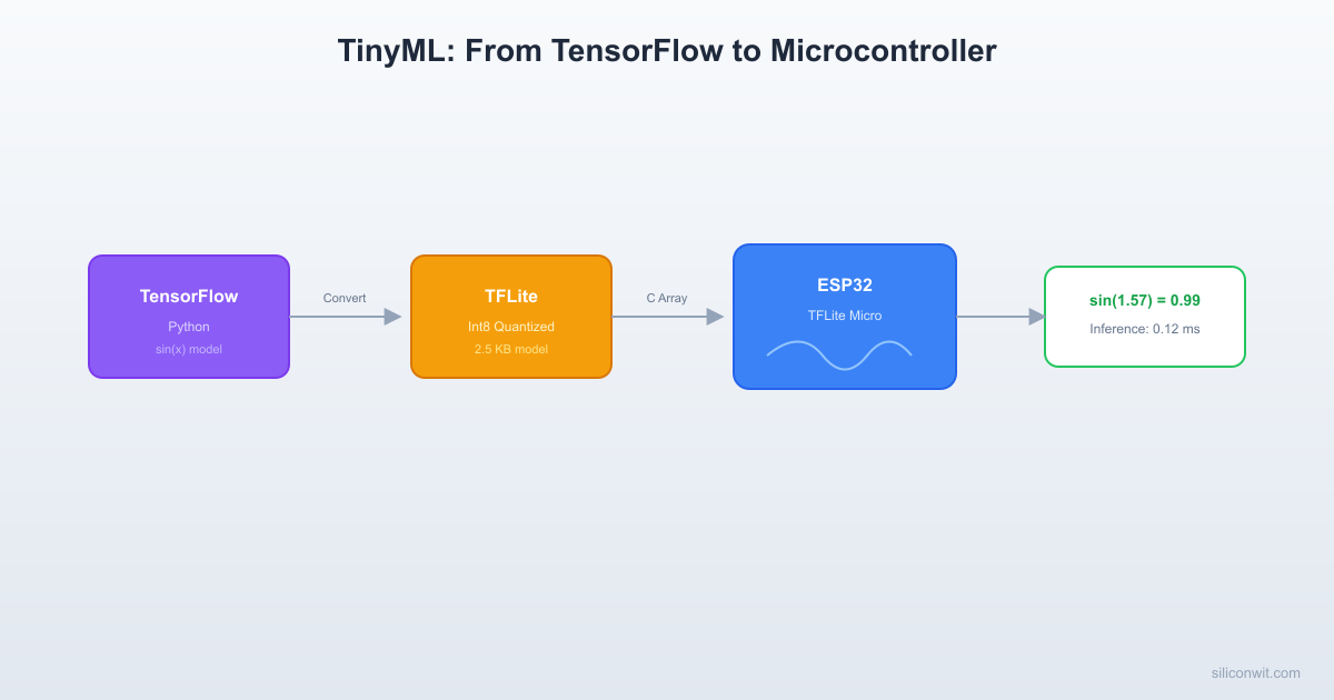
Sending raw sensor data to the cloud for inference adds latency, costs bandwidth, and fails the moment the network goes down. For applications like keyword detection, gesture recognition, or anomaly alerts, even a few hundred milliseconds of round-trip delay can make the system unusable. Running the model directly on the microcontroller eliminates all three problems: inference happens in microseconds, no network is needed, and the data never leaves the device. In this first lesson you will walk through the complete TinyML pipeline: train a sine wave regression model in TensorFlow on your PC, quantize it to int8, convert it to a C array, and deploy it on an ESP32 using TensorFlow Lite for Microcontrollers. By the end you will see predictions printed over serial and measure how fast inference runs on a 240 MHz core. #TinyML #EdgeAI #ESP32
What is TinyML?
TinyML refers to running machine learning inference on microcontrollers and ultra-low-power devices. The key distinction from traditional ML is the hardware budget. A cloud GPU has gigabytes of memory and teraflops of compute. A microcontroller has kilobytes of RAM, hundreds of kilobytes of flash, and clock speeds measured in tens or hundreds of megahertz.
The Core Idea
Train the model on a powerful machine (your laptop, a cloud instance, Edge Impulse). Then compress and convert the trained model into a format that fits inside the MCU’s flash. At runtime, a tiny interpreter loads the model, allocates a small memory arena, and executes inference on live sensor data. The result is a classification label, a regression value, or an anomaly score, produced entirely on-device.
  Cloud ML vs Edge ML  ──────────────────────────────────────────  Cloud ML:  Sensor ──WiFi──► Cloud GPU ──► Result          ~100ms    ~50ms        ~100ms          network   inference    network          Total: ~250ms + connectivity required
  Edge ML (TinyML):  Sensor ──► MCU ──► Result              ~5ms              inference          Total: ~5ms, works offline
Why Run ML on the Edge?
Benefit
Explanation
Low latency
Inference takes milliseconds on-device. No network round-trip.
Connectivity optional
The model is baked into firmware. Core inference works offline, though production systems benefit from cloud connectivity for model updates and escalation (Lesson 9).
Privacy
Raw sensor data never leaves the device. Only results are transmitted.
Low power
A Cortex-M4 running inference at 1 Hz draws single-digit milliamps.
Low cost
A 2 USD MCU replaces a 50 USD SBC or a cloud API subscription.
TinyML Pipeline: Train to Deploy
──────────────────────────────────────────
PC / Cloud MCU (ESP32)
────────── ────────────
1. Collect 5. Flash C array
training data to MCU flash
│ │
2. Train model 6. TFLM interpreter
(TensorFlow) loads model
│ │
3. Quantize 7. Feed live sensor
float32 → int8 data as input
│ │
4. Convert to 8. Get prediction
.tflite → C (class label or
header array regression value)
Hardware Constraints
Before writing any code, internalize the resource budget of common TinyML targets.
MCU
CPU
Clock
Flash
SRAM
FPU
Typical Use
ESP32 (Xtensa LX6)
Dual-core
240 MHz
4 MB
520 KB
Yes
Wi-Fi/BLE + ML
STM32F4 (Cortex-M4F)
Single-core
168 MHz
1 MB
192 KB
Yes
Industrial ML
RPi Pico (Cortex-M0+)
Dual-core
133 MHz
2 MB
264 KB
No
Low-cost ML
nRF52840 (Cortex-M4F)
Single-core
64 MHz
1 MB
256 KB
Yes
BLE + ML
Practical limits for model size:
Flash: your model (as a C array) must fit in flash alongside the firmware. A typical budget is 50 KB to 500 KB for the model.
RAM: the TFLM interpreter needs a “tensor arena” in RAM to hold intermediate activations. Budget 20 KB to 100 KB depending on the model.
Compute: inference time depends on the number of multiply-accumulate operations. Int8 quantized models are 2x to 4x faster than float32 on Cortex-M4 with CMSIS-NN.
The ML Pipeline for Microcontrollers
Collect or generate training data.
For this lesson we generate synthetic sine wave data. In later lessons you will collect real sensor data.
Train a model in TensorFlow (or PyTorch, scikit-learn).
Use standard Python ML tooling on your PC. The model architecture must be small enough to convert.
Convert to TensorFlow Lite (.tflite).
The TFLite converter produces a FlatBuffer binary. Apply post-training quantization (int8) to shrink size and speed up inference.
Convert .tflite to a C array.
The xxd utility (or a Python script) turns the binary into a const unsigned char[] that compiles into firmware.
Write firmware that runs the TFLM interpreter.
Allocate a tensor arena, load the model, invoke the interpreter, and read the output tensor.
Flash, run, and evaluate.
Measure accuracy against ground truth and log inference time.
Project: Sine Wave Predictor on ESP32
We will train a tiny neural network to approximate the function y = sin(x) over the range [0, 2*pi]. This is the canonical “hello world” of TinyML because it requires zero external hardware (just an ESP32 and a serial monitor) and it exercises every step of the pipeline.
Step 1: Train the Sine Model in Python
Create a file called train_sine_model.py on your PC.
train_sine_model.py
# Train a tiny sine wave regression model and export to TFLite (int8)
Espressif maintains esp-tflite-micro as a ready-to-use ESP-IDF component. It includes CMSIS-NN optimized kernels for Xtensa.
Top-Level CMakeLists.txt
sine_predictor/CMakeLists.txt
cmake_minimum_required(VERSION 3.16)
set(EXTRA_COMPONENT_DIRS "components/tfmicro")
include($ENV{IDF_PATH}/tools/cmake/project.cmake)
project(sine_predictor)
Main Component CMakeLists.txt
sine_predictor/main/CMakeLists.txt
idf_component_register(
SRCS "main.cc""sine_model_data.c"
INCLUDE_DIRS "."
REQUIRES esp-tflite-micro
)
Step 4: Firmware (ESP-IDF C with TFLM)
The TFLM C++ API is wrapped here in a C-compatible main.c file. Since TFLM is C++, rename this file to main.cc if your build requires it, or use extern "C" as shown.
main/main.cc
// Sine wave predictor using TensorFlow Lite for Microcontrollers on ESP32
You should see a table printed over serial with 50 data points. Typical results on an ESP32 at 240 MHz:
Metric
Typical Value
Model size (int8 .tflite)
2.4 KB to 3.5 KB
Tensor arena used
~1.2 KB
Average inference time
30 to 80 microseconds
Average absolute error
0.05 to 0.15
The inference time is remarkable. At 50 microseconds per inference, you could run 20,000 predictions per second, far more than any real sensor would need.
Understanding the TFLM Components
The Model (FlatBuffer)
TFLite models use Google’s FlatBuffers serialization format. The .tflite file contains the model architecture (which ops, in what order), the trained weights (quantized to int8), and metadata (tensor shapes, quantization parameters). When you embed this as a C array, it lives in flash. The interpreter reads it directly from flash without copying it to RAM.
The template parameter <3> is the maximum number of ops. Each Add...() call registers a kernel implementation. Only register the ops your model actually uses. This keeps the binary small. If you register AllOpsResolver instead, every kernel gets linked in, adding 100 KB or more to the firmware.
This is a contiguous block of RAM that the interpreter uses for input tensors, output tensors, and all intermediate activation buffers. The alignment matters for SIMD operations. If the arena is too small, AllocateTensors() will fail. If it is too large, you waste RAM. Use interpreter.arena_used_bytes() to find the actual usage and size the arena accordingly.
The Interpreter
The MicroInterpreter is the runtime engine. It:
Parses the FlatBuffer model.
Allocates tensors within the arena.
On each Invoke() call, executes the ops in sequence.
Writes the result to the output tensor.
There is no dynamic memory allocation after AllocateTensors(). This deterministic behavior is critical for real-time embedded systems.
Quantization: Float32 vs Int8
The model we trained in Python used float32 weights and activations. The TFLite converter with representative_dataset performed post-training quantization to int8. Here is what changed:
Property
Float32 Model
Int8 Model
Weight precision
32-bit float
8-bit integer
Model file size
~8 KB
~2.5 KB
Inference speed on ESP32
~120 us
~50 us
RAM for activations
~4 KB
~1.2 KB
Accuracy (MAE)
~0.05
~0.08
The int8 model is smaller, faster, and uses less RAM, at the cost of slightly higher error. For a sine wave, the accuracy difference is negligible. For complex models the trade-off becomes more important, which is why Lesson 4 covers quantization in depth.
Exercises
Exercise 1: Modify the Network
Change the hidden layer sizes from 16 to 8 neurons each. Retrain, convert, and deploy. How does the model size change? How does accuracy change? Find the smallest network that keeps MAE under 0.2.
Exercise 2: Float32 Comparison
Export the model without quantization (remove the representative_dataset and int8 settings from the converter). Deploy the float32 model on ESP32 and compare inference time, arena size, and accuracy against the int8 version.
Exercise 3: Continuous Prediction
Modify the firmware to run inference in a loop at 10 Hz (every 100 ms) and print the results. This simulates a real sensor pipeline where new data arrives continuously.
Exercise 4: Add cos(x)
Modify the training script to predict both sin(x) and cos(x) simultaneously (2 output neurons). Update the firmware to read both outputs. This introduces multi-output regression.
What Comes Next
You now have the complete mental model: train on PC, quantize, convert to C, run on MCU. In the next lesson, you will use Edge Impulse to collect real accelerometer data, train a motion classifier in the cloud, and deploy it back to the ESP32. The pipeline gets more practical, but the core pattern stays the same.
Comments