Logistic regression and decision trees work well when the decision boundary is simple, but they cannot learn features like “this vibration pattern looks abnormal” or “this combination of sensor readings precedes a failure.” Neural networks can, because stacking layers of weighted sums and nonlinear activations lets them build increasingly abstract representations of the input. The catch is that this power comes with complexity: backpropagation, vanishing gradients, and weight initialization all hide behind a single call to model.fit(). In this lesson you will build a neural network from scratch using nothing but NumPy, see every number that flows through it, and train it to solve problems that linear models cannot touch. #NeuralNetworks #Backpropagation #NumPy
A Single Neuron
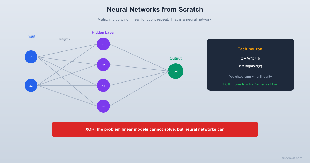
Every neural network starts with this building block: a neuron takes inputs, multiplies each by a weight, adds a bias, and passes the result through an activation function.
  A Single Neuron  ──────────────────────────────────────────  Inputs       Weights      Sum + Bias    Activation  ──────       ───────      ──────────    ──────────  x1 ─── w1 ──┐               ├──► z = w1*x1 + w2*x2 + b ──► a = f(z)  x2 ─── w2 ──┘
  f(z) is a nonlinear function (sigmoid, ReLU, etc.)  Without f(z), stacking layers would collapse to a single linear transform.
Why Nonlinearity Matters
If every neuron were just a linear function (output = weights * inputs + bias), then stacking 100 layers would still produce a linear function. You could replace the entire network with a single layer. Nonlinear activation functions break this limitation and allow networks to learn curved decision boundaries, thresholds, and complex patterns.
import numpy as np
np.random.seed(42)
# A single neuron
defsingle_neuron(x, w, b):
"""Weighted sum + bias, then sigmoid activation."""
z = np.dot(x, w) + b
a =1/ (1+ np.exp(-z)) # sigmoid
return a
# Two inputs
x = np.array([0.5, 0.8])
w = np.array([0.3, -0.1])
b =0.2
output =single_neuron(x, w, b)
print(f"Inputs: {x}")
print(f"Weights: {w}")
print(f"Bias: {b}")
print(f"Weighted sum: {np.dot(x, w)+ b:.4f}")
print(f"After sigmoid: {output:.4f}")
Expected output:
Inputs: [0.5 0.8]
Weights: [0.3 -0.1]
Bias: 0.2
Weighted sum: 0.2700
After sigmoid: 0.5671
The sigmoid squished the value 0.27 to 0.5671 (always between 0 and 1). That is the entire computation inside one neuron.
Activation Functions
Two activation functions cover most practical cases.
import numpy as np
np.random.seed(42)
defsigmoid(z):
return1/ (1+ np.exp(-z))
defsigmoid_derivative(a):
"""Derivative of sigmoid, given the output a = sigmoid(z)."""
Sigmoid squishes any value into (0, 1). Useful for output layers where you want a probability. ReLU (Rectified Linear Unit) passes positive values through and zeros out negatives. It is simple, fast, and avoids the vanishing gradient problem that plagues deep sigmoid networks.
Why ReLU Replaced Sigmoid in Hidden Layers
Look at the sigmoid derivative row above: the largest value is 0.25, reached only at z = 0. For any large positive or negative input, the derivative collapses toward zero. During backpropagation, gradients are multiplied layer by layer. In a network with 10 sigmoid layers, the gradient at the first layer can be scaled by (0.25)^10, about 1 in a million. The early layers stop learning. This is the vanishing gradient problem.
ReLU’s derivative is 1 for any positive input (and 0 otherwise), so it does not attenuate gradients as they flow backwards. This is the single biggest reason deep networks started working in the 2010s. Use ReLU in hidden layers by default; save sigmoid for output layers where you need a probability.
The XOR Problem
XOR is the classic test: the output is 1 when exactly one input is 1, and 0 otherwise. A single layer (linear model) cannot solve this because the classes are not linearly separable. A two-layer network can.
XOR Truth Table Why Linear Models Fail
──────────────── ──────────────────────
x1 x2 │ y x2
0 0 │ 0 1 ──── ● (0,1)=1 ○ (1,1)=0
0 1 │ 1 │
1 0 │ 1 │ No single straight line
1 1 │ 0 │ separates ● from ○
0 ──── ○ (0,0)=0 ● (1,0)=1
0 1 x1
A Note on Weight Initialization
The code below initializes weights as small random Gaussians with a hand-picked scale. That is fine for this 2-layer toy, but if you try to stack 10 ReLU layers with the same scheme, signals either blow up or die out as they travel through the network. Modern frameworks use principled schemes that set the initial variance based on the fan-in and fan-out of each layer:
Xavier / Glorot initialization: pairs well with tanh and sigmoid.
He / Kaiming initialization: pairs well with ReLU and its variants.
In PyTorch these are torch.nn.init.xavier_uniform_() and torch.nn.init.kaiming_normal_(). You do not need to memorize the formulas; you need to know that “I just pick small random numbers” stops working once the network is deep, and to use the initializer that matches your activation.
The network learned XOR. A linear model would be stuck at ~50% accuracy on this problem forever.
Understanding Backpropagation
Backpropagation is the chain rule applied backwards through the network. Each layer computes: “How much did my weights contribute to the total error?”
Forward pass: compute predictions layer by layer.
Compute loss: how far off are the predictions? (MSE in our case.)
Output layer gradient: compute how the loss changes with respect to the output weights. This uses the derivative of the sigmoid and the derivative of MSE.
Hidden layer gradient: propagate the error backward through the output weights and multiply by the derivative of ReLU. This tells each hidden neuron how much it contributed to the error.
Update weights: subtract learning_rate * gradient from each weight. Repeat.
Now a more practical problem. Given temperature and vibration readings from an industrial sensor, classify each reading as normal (0), warning (1), or critical (2).
Predicted: Normal (99.01%) | Actual: Normal | correct
...
The network architecture uses softmax in the output layer for multi-class classification. Softmax converts raw scores into probabilities that sum to 1 across all classes.
3-Class Sensor Classification Network
──────────────────────────────────────────
Input (2) Hidden (16) Output (3)
───────── ─────────── ──────────
Temperature ──┬── h1 ┌─ Normal (softmax)
├── h2 │
├── h3 ────────────├─ Warning (softmax)
├── ... │
└── h16 └─ Critical (softmax)
Vibration ────┘
ReLU Probabilities sum to 1.0
Key Takeaways
A Neuron
Weighted sum + bias + activation function. That is the entire computation. Everything else is just organizing neurons into layers.
Forward Pass
Input flows through each layer: multiply by weights, add bias, apply activation. The output of one layer is the input to the next.
Backpropagation
The chain rule applied backwards. Each layer computes its gradient, which tells us how to adjust its weights to reduce the loss.
What Frameworks Do
TensorFlow and PyTorch do exactly what you just coded, but optimized for GPUs, with automatic differentiation, and scaled to millions of parameters. Now you know what happens inside.
Regularizers You Will Meet Next
Real networks fight overfitting with two standard tools you did not need here. Dropout randomly zeros a fraction of activations at each training step, forcing the network to not rely on any single unit. Batch normalization rescales activations using running mini-batch statistics, stabilizing training and allowing higher learning rates. Both are one-liners in PyTorch and Keras, and both live inside frameworks rather than in the raw math.
Now you know what TensorFlow does internally. It is this: matrix multiplications, nonlinear activations, loss computation, and gradient updates, optimized and scaled to billions of parameters.
Comments