Feedback and Control Systems

Modified: Mar. 15, 2026

Published: Mar. 9, 2026

Become Contributor Expert Support

You want your room at 22 degrees. The heater runs, the temperature rises, and when it reaches 22 you turn the heater off. But by the time the room responds, it has overshot to 24. So you wait, it drops, undershoots to 20, and you turn the heater on again. This oscillation is what happens when feedback is done badly. Done well, feedback is the single most powerful idea in engineering: it lets imprecise components produce precise results, and it lets simple systems handle complex, unpredictable environments. #ControlSystems #PID #FeedbackControl

Open-Loop vs. Closed-Loop Control

Open-loop control sets the input and hopes for the best. You set the heater to 50% power because you calculated that should maintain 22 degrees. If the window is open, if the sun comes out, if someone leaves the door ajar, the temperature drifts and the controller does nothing about it.

Closed-loop control measures the output and adjusts the input to correct errors. It does not need to know about the window or the sun. It sees that the temperature is too low and increases the heater power. It sees the temperature is too high and decreases it. The feedback loop makes the system self-correcting.

Open-loop:
  Desired temp --> [Controller] --> [Heater] --> Room temp
  (no feedback, no correction)

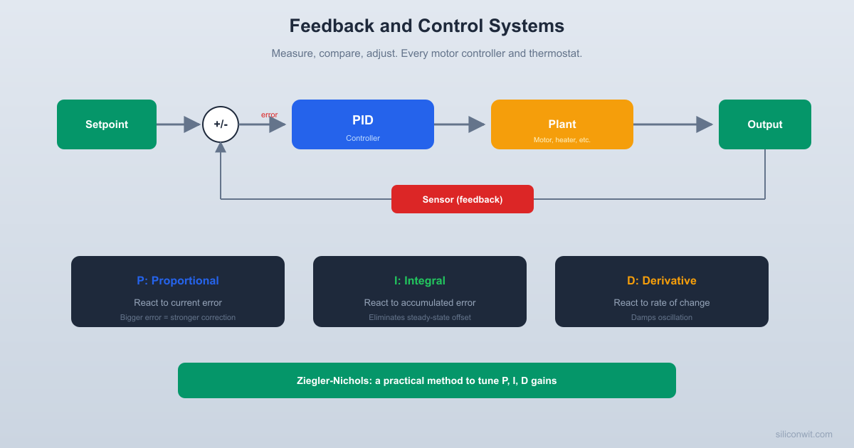
Closed-loop:
  Desired temp -->(+)-->[Controller]-->[Heater]-->[Room]--+-- Room temp
                   ^                                       |
                   |          error = desired - actual      |
                   +----------[Sensor]<--------------------+

The closed-loop diagram is the most important diagram in control engineering. Every feedback system, from a thermostat to a self-driving car, follows this structure.

Cruise control in your car is a textbook example: it measures your speed (sensor), compares it to the speed you set (setpoint), and adjusts the throttle (output) to minimize the difference. Your body works the same way: the hypothalamus measures your core temperature, and if it deviates from 37 degrees C, it triggers sweating (too hot) or shivering (too cold) to bring it back.

The Error Signal

The error is the difference between what you want (the setpoint or reference) and what you have (the measured output):

where is the reference and is the output. The controller’s job is to drive toward zero. Everything else is details about how to do that effectively.

Proportional Control: The Simplest Controller

The most obvious controller: make the control effort proportional to the error.

If the temperature is 2 degrees below the setpoint, apply twice as much heat as when it is 1 degree below. The constant is the proportional gain.

Why P-Only Control Has Steady-State Error

Proportional control has a fundamental limitation. The controller output is . For the heater to produce any heat, the error must be nonzero. The system settles to a state where the error is just large enough to generate the control effort needed to balance the heat losses. This permanent offset is called steady-state error (or droop).

Increasing reduces the steady-state error (because less error is needed to produce the same effort) but makes the system more aggressive, leading to oscillation and instability.

import numpy as np
import matplotlib.pyplot as plt

def simulate_p_control(Kp, setpoint, t_end=100, dt=0.1):
    """Simulate P control of a first-order thermal system.
    Plant: dT/dt = -0.1*(T - T_ambient) + 0.05*u
    """
    T_ambient = 15.0
    N = int(t_end / dt)
    t = np.zeros(N)
    T = np.zeros(N)
    u = np.zeros(N)
    T[0] = T_ambient  # start at ambient

    for i in range(N - 1):
        error = setpoint - T[i]
        u[i] = np.clip(Kp * error, 0, 100)  # 0-100% heater
        dTdt = -0.1 * (T[i] - T_ambient) + 0.05 * u[i]
        T[i+1] = T[i] + dTdt * dt
        t[i+1] = t[i] + dt

    u[-1] = u[-2]
    return t, T, u

setpoint = 25.0
fig, (ax1, ax2) = plt.subplots(2, 1, figsize=(10, 6), sharex=True)

for Kp in [5, 15, 50]:
    t, T, u = simulate_p_control(Kp, setpoint)
    ax1.plot(t, T, linewidth=1.5, label=f'Kp={Kp}')
    ax2.plot(t, u, linewidth=1, label=f'Kp={Kp}')

ax1.axhline(setpoint, color='k', linestyle='--', alpha=0.5, label='Setpoint')
ax1.set_ylabel('Temperature (C)')
ax1.set_title('Proportional Control: Effect of Gain')
ax1.legend()
ax1.grid(True, alpha=0.3)

ax2.set_ylabel('Heater Power (%)')
ax2.set_xlabel('Time (s)')
ax2.grid(True, alpha=0.3)
ax2.legend()

plt.tight_layout()
plt.show()

Notice: none of the P-only responses reach the setpoint exactly. The gap is the steady-state error.

PI Control: Eliminating Steady-State Error

The fix for steady-state error: add an integral term that accumulates the error over time.

Even a tiny, persistent error will eventually build up a large integral, generating enough control effort to eliminate the offset completely. The integral “remembers” past errors and keeps pushing until the error reaches zero.

The Cost of Integral Action

The integral term introduces a new problem: overshoot. The integral accumulates while the error is positive (approaching the setpoint). By the time the temperature reaches the setpoint, the integral is large and positive, so the controller keeps pushing. The temperature overshoots, and the integral must wind down before the system settles.

This is called integral windup: the integral builds up to a large value during a sustained error and takes time to unwind. In practice, you clamp (limit) the integral term to prevent excessive windup.

Python: PI Control Simulation

import numpy as np
import matplotlib.pyplot as plt

def simulate_pi_control(Kp, Ki, setpoint, t_end=200, dt=0.1):
    """Simulate PI control of a first-order thermal system."""
    T_ambient = 15.0
    N = int(t_end / dt)
    t = np.zeros(N)
    T = np.zeros(N)
    u = np.zeros(N)
    T[0] = T_ambient
    integral = 0.0

    for i in range(N - 1):
        error = setpoint - T[i]
        integral += error * dt
        integral = np.clip(integral, -500, 500)  # anti-windup

        u[i] = np.clip(Kp * error + Ki * integral, 0, 100)
        dTdt = -0.1 * (T[i] - T_ambient) + 0.05 * u[i]
        T[i+1] = T[i] + dTdt * dt
        t[i+1] = t[i] + dt

    u[-1] = u[-2]
    return t, T, u

setpoint = 25.0
fig, ax = plt.subplots(figsize=(10, 5))

# P-only for reference
t, T, _ = simulate_p_control(15, setpoint, t_end=200)
ax.plot(t, T, 'b--', linewidth=1, label='P only (Kp=15)')

# PI with different Ki
for Ki in [0.05, 0.2, 0.8]:
    t, T, _ = simulate_pi_control(15, Ki, setpoint, t_end=200)
    ax.plot(t, T, linewidth=1.5, label=f'PI (Kp=15, Ki={Ki})')

ax.axhline(setpoint, color='k', linestyle='--', alpha=0.5, label='Setpoint')
ax.set_xlabel('Time (s)')
ax.set_ylabel('Temperature (C)')
ax.set_title('PI Control: Integral Action Removes Steady-State Error')
ax.legend()
ax.grid(True, alpha=0.3)
plt.tight_layout()
plt.show()

PID Control: Adding Damping

The derivative term looks at the rate of change of the error. If the temperature is approaching the setpoint rapidly, the derivative is large and negative. The derivative term reduces the control effort before the system reaches the setpoint, damping the overshoot.

The Derivative Problem: Noise Amplification

The derivative term computes the rate of change of the error. If the sensor signal is noisy, the derivative amplifies that noise dramatically. A noisy temperature reading bouncing by 0.1 degrees produces huge spikes in the derivative.

Two practical solutions:

1. Apply a low-pass filter to the derivative term (or to the measurement)
2. Differentiate the process variable instead of the error: instead of . This avoids the derivative spike that occurs when the setpoint changes suddenly.

Python: Full PID Controller

import numpy as np
import matplotlib.pyplot as plt

def simulate_pid(Kp, Ki, Kd, setpoint, t_end=200, dt=0.1,
                 disturbance_time=None, disturbance_value=0):
    """Simulate PID control of a first-order thermal system."""
    T_ambient = 15.0
    N = int(t_end / dt)
    t = np.zeros(N)
    T = np.zeros(N)
    u = np.zeros(N)
    T[0] = T_ambient
    integral = 0.0
    prev_error = setpoint - T[0]

    for i in range(N - 1):
        error = setpoint - T[i]

        # PID terms
        integral += error * dt
        integral = np.clip(integral, -500, 500)  # anti-windup

        derivative = (error - prev_error) / dt
        prev_error = error

        u[i] = np.clip(Kp * error + Ki * integral + Kd * derivative,
                       0, 100)

        # Plant dynamics with optional disturbance
        dist = 0
        if disturbance_time and t[i] > disturbance_time:
            dist = disturbance_value

        dTdt = -0.1 * (T[i] - T_ambient) + 0.05 * u[i] + dist
        T[i+1] = T[i] + dTdt * dt
        t[i+1] = t[i] + dt

    u[-1] = u[-2]
    return t, T, u

setpoint = 25.0

# Compare P, PI, PID
configs = [
    ('P only',   15, 0,    0),
    ('PI',       15, 0.2,  0),
    ('PID',      15, 0.2,  5),
]

fig, (ax1, ax2) = plt.subplots(2, 1, figsize=(10, 7), sharex=True)

for label, Kp, Ki, Kd in configs:
    t, T, u = simulate_pid(Kp, Ki, Kd, setpoint, t_end=150)
    ax1.plot(t, T, linewidth=1.5, label=label)
    ax2.plot(t, u, linewidth=1, label=label)

ax1.axhline(setpoint, color='k', linestyle='--', alpha=0.5, label='Setpoint')
ax1.set_ylabel('Temperature (C)')
ax1.set_title('P vs PI vs PID Control')
ax1.legend()
ax1.grid(True, alpha=0.3)

ax2.set_ylabel('Heater Power (%)')
ax2.set_xlabel('Time (s)')
ax2.legend()
ax2.grid(True, alpha=0.3)

plt.tight_layout()
plt.show()

Tuning: The Ziegler-Nichols Method

Choosing , , and is the practical challenge. The Ziegler-Nichols method gives you a starting point based on the system’s response.

Ultimate Gain Method

1. Set and (P-only control)

2. Increase gradually until the system oscillates with constant amplitude (neither growing nor decaying). This is the ultimate gain

3. Measure the ultimate period of the oscillation

4. Set the PID gains according to the table below

These values are a starting point, not the final answer. They typically produce a response with about 25% overshoot. From there, you tune by hand: reduce if there is too much oscillation, increase if steady-state error persists, increase if overshoot is excessive.

Python: Finding Ultimate Gain

import numpy as np
import matplotlib.pyplot as plt

def simulate_for_tuning(Kp, t_end=100, dt=0.05):
    """Simulate P control to find ultimate gain and period."""
    T_ambient = 15.0
    setpoint = 25.0
    N = int(t_end / dt)
    t = np.zeros(N)
    T = np.zeros(N)
    T[0] = T_ambient

    for i in range(N - 1):
        error = setpoint - T[i]
        u = np.clip(Kp * error, 0, 100)
        dTdt = -0.1 * (T[i] - T_ambient) + 0.05 * u
        T[i+1] = T[i] + dTdt * dt
        t[i+1] = t[i] + dt

    return t, T

# Try increasing Kp values
fig, axes = plt.subplots(2, 2, figsize=(10, 6))
gains = [10, 30, 55, 80]

for ax, Kp in zip(axes.flat, gains):
    t, T = simulate_for_tuning(Kp)
    ax.plot(t, T, 'b-', linewidth=1)
    ax.axhline(25, color='k', linestyle='--', alpha=0.5)
    ax.set_title(f'Kp = {Kp}')
    ax.set_ylim(10, 40)
    ax.grid(True, alpha=0.3)
    ax.set_xlabel('Time (s)')
    ax.set_ylabel('Temp (C)')

plt.suptitle('Finding Ultimate Gain: Increasing Kp', fontsize=12)
plt.tight_layout()
plt.show()

Stability: What Happens When the Gain Is Too High

Feedback can make a system better or worse. If the gain is too high, the controller overreacts to every small disturbance. Each correction causes a larger error in the opposite direction. The oscillations grow until the system saturates or something breaks.

The boundary between stable and unstable is not gradual. A system can be perfectly stable at and wildly unstable at . This sensitivity is why control system design requires analysis, not guesswork.

Gain Margin and Phase Margin

Two measures of “how close to instability”:

• Gain margin: how much you can increase the gain before the system goes unstable. A gain margin of 6 dB means you can roughly double the gain before instability.
• Phase margin: how much additional phase lag the system can tolerate. A phase margin of 45 degrees is a common design target.

These are advanced topics from frequency-domain control theory, but the intuition is straightforward: both measure how much room for error you have before the feedback loop starts amplifying errors instead of correcting them.

Practical Applications

Disturbance Rejection: The Real Test

A controller that reaches the setpoint in calm conditions is not finished. The real test is how it handles disturbances: someone opens the oven door, the motor load changes, a gust of wind hits the drone.

import numpy as np
import matplotlib.pyplot as plt

setpoint = 25.0

# Simulate with a disturbance at t=100 (like opening a window)
fig, ax = plt.subplots(figsize=(10, 5))

configs = [
    ('P only',   15, 0,    0),
    ('PI',       15, 0.2,  0),
    ('PID',      15, 0.2,  5),
]

for label, Kp, Ki, Kd in configs:
    t, T, u = simulate_pid(Kp, Ki, Kd, setpoint, t_end=300,
                           disturbance_time=100, disturbance_value=-0.3)
    ax.plot(t, T, linewidth=1.5, label=label)

ax.axhline(setpoint, color='k', linestyle='--', alpha=0.3)
ax.axvline(100, color='gray', linestyle=':', alpha=0.5)
ax.annotate('Disturbance\n(window opens)', xy=(100, 23),
            fontsize=9, ha='center')
ax.set_xlabel('Time (s)')
ax.set_ylabel('Temperature (C)')
ax.set_title('Disturbance Rejection: P vs PI vs PID')
ax.legend()
ax.grid(True, alpha=0.3)
plt.tight_layout()
plt.show()

The P-only controller reaches a new (wrong) steady state after the disturbance. The PI and PID controllers eventually return to the setpoint, but PID returns faster with less overshoot. This is where the derivative term earns its keep.

Implementation Checklist

When implementing a PID controller on a real system:

1. Saturate the output. The actuator has physical limits (0 to 100% power, for example). Clamp the PID output to these limits.

2. Implement anti-windup. When the output saturates, stop accumulating the integral. Otherwise, the integral grows unbounded and causes large overshoot when the system exits saturation.

3. Filter the derivative. Apply a low-pass filter to the derivative term (or to the measurement) to suppress noise amplification. A simple first-order filter with time constant works well.

4. Use a fixed sample rate. The PID algorithm assumes uniform time steps. Use a timer interrupt to ensure consistent sample intervals.

5. Start conservative. Begin with low gains and increase gradually. A system that oscillates can break things. A system that responds slowly is merely annoying.

Exercises

1. P-only steady-state error. Analytically, for the thermal system used in this lesson (, ), derive the steady-state temperature as a function of and the setpoint. Verify your formula against the simulation.

2. Ziegler-Nichols tuning. For the thermal system, find the ultimate gain and ultimate period by simulation. Apply the Ziegler-Nichols PID formulas. Simulate the result. Does the response have approximately 25% overshoot as expected?

3. Setpoint tracking. Modify the PID simulation to follow a setpoint that changes over time: hold at 25 C for 50 seconds, ramp to 35 C over 20 seconds, hold at 35 C. How does the controller handle the ramp?

4. Noise sensitivity. Add Gaussian noise (standard deviation 0.2 C) to the temperature measurement in the PID simulation. Compare the control signal with and without derivative action. Then add a first-order low-pass filter to the derivative and observe the improvement.

5. Cascaded control. Implement a position controller for a DC motor (second-order system: ). Use an inner PID loop for velocity and an outer P loop for position. Compare with a single PID loop for position directly.

References

• Astrom, K. J. and Murray, R. M. (2021). Feedback Systems: An Introduction for Scientists and Engineers. Princeton University Press. Free online: fbsbook.org
• Franklin, G. F. et al. (2018). Feedback Control of Dynamic Systems. Pearson.
• Bennett, S. (1993). A History of Control Engineering, 1930-1955. IEE. Fascinating history of how PID control was developed for process industries.