How Models Learn: Gradient Descent

  The Loss Landscape
  ──────────────────────────────────────────────

  Loss
    |
    |  *  Start here
    |   \
    |    \    The gradient points UPHILL
    |     \   (toward increasing loss).
    |      \
    |       \  You step in the OPPOSITE
    |        \ direction (downhill).
    |         \
    |          \___
    |              \___
    |                  \___*  Minimum
    |
    +─────────────────────────────────────
              Parameter value (w)

  Update rule:
    w_new = w_old - learning_rate * gradient

  That single equation is the engine behind:
    - Linear regression
    - Logistic regression
    - Neural networks
    - Deep learning
    - Transformer models (GPT, etc.)

import numpy as np

np.random.seed(42)

# ── Generate data: y = 3x + 7 + noise ──
n = 100
x = np.random.uniform(0, 10, n)
y = 3 * x + 7 + np.random.randn(n) * 2

# ── Initialize parameters randomly ──
w = np.random.randn()  # weight (slope)
b = np.random.randn()  # bias (intercept)
lr = 0.01              # learning rate
epochs = 200           # number of iterations

print(f"True parameters:    w = 3.000, b = 7.000")
print(f"Initial parameters: w = {w:.3f}, b = {b:.3f}")
print()

# ── Gradient descent loop ──
losses = []
for epoch in range(epochs):
    # Forward pass: compute predictions
    y_pred = w * x + b

    # Compute loss (MSE)
    loss = np.mean((y - y_pred) ** 2)
    losses.append(loss)

    # Compute gradients
    dw = -2 * np.mean(x * (y - y_pred))  # gradient w.r.t. weight
    db = -2 * np.mean(y - y_pred)         # gradient w.r.t. bias

    # Update parameters (step downhill)
    w = w - lr * dw
    b = b - lr * db

    # Print progress every 20 epochs
    if epoch % 20 == 0 or epoch == epochs - 1:
        print(f"Epoch {epoch:>4d}: loss = {loss:.4f}, w = {w:.4f}, b = {b:.4f}")

print(f"\nFinal parameters: w = {w:.3f}, b = {b:.3f}")
print(f"True parameters:  w = 3.000, b = 7.000")
print(f"Final loss: {losses[-1]:.4f}")

import numpy as np
import matplotlib.pyplot as plt

np.random.seed(42)

# ── Generate data ──
n = 100
x = np.random.uniform(0, 10, n)
y = 3 * x + 7 + np.random.randn(n) * 2

# ── Gradient descent with history tracking ──
w = np.random.randn()
b = np.random.randn()
lr = 0.01
epochs = 200

losses = []
w_history = [w]
b_history = [b]

for epoch in range(epochs):
    y_pred = w * x + b
    loss = np.mean((y - y_pred) ** 2)
    losses.append(loss)

    dw = -2 * np.mean(x * (y - y_pred))
    db = -2 * np.mean(y - y_pred)

    w = w - lr * dw
    b = b - lr * db
    w_history.append(w)
    b_history.append(b)

# ── Plot 1: Loss Curve ──
fig, axes = plt.subplots(1, 3, figsize=(16, 5))

axes[0].plot(losses, color='steelblue', linewidth=2)
axes[0].set_xlabel('Epoch')
axes[0].set_ylabel('MSE Loss')
axes[0].set_title('Loss Decreases Over Training')
axes[0].grid(True, alpha=0.3)
axes[0].set_yscale('log')

# ── Plot 2: Parameter Convergence ──
axes[1].plot(w_history, label=f'w (converges to ~3.0)', color='steelblue', linewidth=2)
axes[1].plot(b_history, label=f'b (converges to ~7.0)', color='tomato', linewidth=2)
axes[1].axhline(y=3.0, color='steelblue', linestyle='--', alpha=0.3)
axes[1].axhline(y=7.0, color='tomato', linestyle='--', alpha=0.3)
axes[1].set_xlabel('Epoch')
axes[1].set_ylabel('Parameter Value')
axes[1].set_title('Parameters Converge to True Values')
axes[1].legend()
axes[1].grid(True, alpha=0.3)

# ── Plot 3: Line Fitting Animation (snapshots) ──
x_line = np.linspace(0, 10, 100)
snapshot_epochs = [0, 5, 20, 50, 199]

axes[2].scatter(x, y, alpha=0.3, s=10, color='gray', label='Data')
colors = plt.cm.viridis(np.linspace(0, 1, len(snapshot_epochs)))

for i, ep in enumerate(snapshot_epochs):
    w_snap = w_history[ep]
    b_snap = b_history[ep]
    y_line = w_snap * x_line + b_snap
    axes[2].plot(x_line, y_line, color=colors[i], linewidth=2,
                 label=f'Epoch {ep}: w={w_snap:.2f}, b={b_snap:.2f}')

axes[2].set_xlabel('x')
axes[2].set_ylabel('y')
axes[2].set_title('Line Fitting Over Training')
axes[2].legend(fontsize=7)
axes[2].grid(True, alpha=0.3)

plt.tight_layout()
plt.savefig('gradient_descent_visualization.png', dpi=100)
plt.show()
print("Plot saved as gradient_descent_visualization.png")
print("\nLeft: the loss drops sharply in early epochs, then levels off.")
print("Middle: both parameters converge to their true values.")
print("Right: the line starts random and rotates into place.")

import numpy as np
import matplotlib.pyplot as plt

np.random.seed(42)

# ── Generate data ──
n = 100
x = np.random.uniform(0, 10, n)
y = 3 * x + 7 + np.random.randn(n) * 2

# ── Try different learning rates ──
learning_rates = [0.0001, 0.01, 0.05, 0.1]
epochs = 200

fig, axes = plt.subplots(2, 2, figsize=(12, 10))
axes = axes.flatten()

for ax, lr in zip(axes, learning_rates):
    w = np.random.randn()
    b = np.random.randn()
    losses = []
    diverged = False

    for epoch in range(epochs):
        y_pred = w * x + b
        loss = np.mean((y - y_pred) ** 2)

        if np.isnan(loss) or loss > 1e10:
            diverged = True
            losses.append(losses[-1] if losses else 1e10)
            break

        losses.append(loss)
        dw = -2 * np.mean(x * (y - y_pred))
        db = -2 * np.mean(y - y_pred)
        w = w - lr * dw
        b = b - lr * db

    ax.plot(losses, color='steelblue', linewidth=2)
    ax.set_xlabel('Epoch')
    ax.set_ylabel('MSE Loss')
    ax.grid(True, alpha=0.3)

    if diverged:
        ax.set_title(f'lr = {lr}: DIVERGED (too large!)', color='red')
    elif losses[-1] > 10:
        ax.set_title(f'lr = {lr}: Too slow (loss = {losses[-1]:.1f})')
    else:
        ax.set_title(f'lr = {lr}: Final loss = {losses[-1]:.4f}')

    ax.set_yscale('log')

plt.suptitle('Effect of Learning Rate on Training', fontsize=14, y=1.01)
plt.tight_layout()
plt.savefig('learning_rate_comparison.png', dpi=100)
plt.show()

print("Learning rate effects:")
print(f"  lr = 0.0001: Too small. The model barely moves in 200 epochs.")
print(f"  lr = 0.01:   Good. Converges smoothly.")
print(f"  lr = 0.05:   Faster convergence but may oscillate.")
print(f"  lr = 0.1:    May overshoot and diverge (loss explodes).")
print(f"\nPlot saved as learning_rate_comparison.png")

  Learning Rate: Too Small vs Too Large
  ──────────────────────────────────────────────

  Too small (lr = 0.0001):
  Loss
    |*****.............................
    |     ****........................
    |         ****....................
    |             **** (barely moving)
    +─────────────────────────────────
                Epochs

  Just right (lr = 0.01):
  Loss
    |*
    | *
    |  **
    |    ****
    |        ********************************
    +─────────────────────────────────
                Epochs

  Too large (lr = 0.1):
  Loss
    |    *         *         *
    |   * *       * *       * *
    |  *   *     *   *     *   *
    | *     *   *     *   *     *
    |*       * *       * *       (oscillating or diverging)
    +─────────────────────────────────
                Epochs

  Gradient Descent as a Feedback Loop
  ──────────────────────────────────────────────

  PID Controller:
    error = setpoint - measurement
    output = Kp * error + Ki * integral(error) + Kd * derivative(error)
    actuator adjusts based on output
    repeat

  Gradient Descent:
    error = loss (how wrong the model is)
    gradient = direction of steepest increase in error
    parameters -= learning_rate * gradient
    repeat

  The parallels:
    error signal    <-->  loss function
    controller gain <-->  learning rate
    actuator output <-->  parameter update
    plant response  <-->  new predictions

  Gradient descent is a proportional controller (P-only)
  where the gain is the learning rate and the error signal
  is the gradient. Variants like Adam add momentum (similar
  to the I and D terms) for better convergence.

import numpy as np
import matplotlib.pyplot as plt

np.random.seed(42)

# ── Generate multi-feature data ──
# True relationship: y = 2*x1 + (-1)*x2 + 0.5*x3 + 5 + noise
n = 200
X = np.random.randn(n, 3)
w_true = np.array([2.0, -1.0, 0.5])
b_true = 5.0
y = X @ w_true + b_true + np.random.randn(n) * 0.5

# ── Feature scaling (important for gradient descent) ──
X_mean = X.mean(axis=0)
X_std = X.std(axis=0)
X_scaled = (X - X_mean) / X_std

# ── Gradient descent ──
w = np.random.randn(3)
b = 0.0
lr = 0.05
epochs = 300

losses = []

print(f"True parameters:    w = {w_true}, b = {b_true:.1f}")
print(f"Initial parameters: w = [{w[0]:.3f}, {w[1]:.3f}, {w[2]:.3f}], b = {b:.3f}")
print()

for epoch in range(epochs):
    # Forward pass
    y_pred = X_scaled @ w + b

    # Loss
    loss = np.mean((y - y_pred) ** 2)
    losses.append(loss)

    # Gradients (vectorized)
    error = y - y_pred
    dw = -2 / n * (X_scaled.T @ error)   # shape: (3,)
    db = -2 / n * np.sum(error)           # scalar

    # Update
    w = w - lr * dw
    b = b - lr * db

    if epoch % 50 == 0 or epoch == epochs - 1:
        print(f"Epoch {epoch:>4d}: loss = {loss:.4f}, w = [{w[0]:.3f}, {w[1]:.3f}, {w[2]:.3f}], b = {b:.3f}")

# ── Unscale weights to compare with true values ──
w_unscaled = w / X_std
b_unscaled = b - np.sum(w * X_mean / X_std)

print(f"\nFinal (unscaled): w = [{w_unscaled[0]:.3f}, {w_unscaled[1]:.3f}, {w_unscaled[2]:.3f}], b = {b_unscaled:.3f}")
print(f"True:             w = [{w_true[0]:.3f}, {w_true[1]:.3f}, {w_true[2]:.3f}], b = {b_true:.3f}")

# ── Plot loss curve ──
plt.figure(figsize=(8, 5))
plt.plot(losses, color='steelblue', linewidth=2)
plt.xlabel('Epoch')
plt.ylabel('MSE Loss')
plt.title('Multivariate Gradient Descent: Loss Curve')
plt.grid(True, alpha=0.3)
plt.yscale('log')
plt.tight_layout()
plt.savefig('multivariate_gd_loss.png', dpi=100)
plt.show()
print("\nPlot saved as multivariate_gd_loss.png")

  Batch vs Stochastic vs Mini-Batch
  ──────────────────────────────────────────────

  Batch Gradient Descent:
    Use ALL n samples to compute the gradient.
    + Stable, smooth convergence.
    - Slow for large datasets (must process everything each step).

  Stochastic Gradient Descent (SGD):
    Use ONE random sample to compute the gradient.
    + Very fast per step.
    - Noisy, zig-zag path toward the minimum.
    + Noise can help escape local minima.

  Mini-Batch Gradient Descent:
    Use a random subset of B samples (typically B = 32 or 64).
    + Compromise: faster than batch, smoother than SGD.
    + Most common in practice (neural network training).

  All three converge to the same minimum (in convex problems).
  Mini-batch is the standard choice for most ML training.

import numpy as np
import matplotlib.pyplot as plt

np.random.seed(42)

# ── Generate data ──
n = 200
x = np.random.uniform(0, 10, n)
y = 3 * x + 7 + np.random.randn(n) * 2

# ── Batch Gradient Descent ──
def run_gd(x, y, mode='batch', batch_size=32, lr=0.01, epochs=100):
    """Run gradient descent in batch, stochastic, or mini-batch mode."""
    np.random.seed(42)
    w, b = np.random.randn(), np.random.randn()
    losses = []

    for epoch in range(epochs):
        # Full loss for tracking (always computed on all data)
        y_pred_full = w * x + b
        losses.append(np.mean((y - y_pred_full) ** 2))

        if mode == 'batch':
            # Use all data
            x_batch, y_batch = x, y
        elif mode == 'sgd':
            # Use one random sample
            idx = np.random.randint(0, len(x))
            x_batch, y_batch = x[idx:idx+1], y[idx:idx+1]
        elif mode == 'mini-batch':
            # Use a random subset
            idx = np.random.choice(len(x), batch_size, replace=False)
            x_batch, y_batch = x[idx], y[idx]

        y_pred = w * x_batch + b
        dw = -2 * np.mean(x_batch * (y_batch - y_pred))
        db = -2 * np.mean(y_batch - y_pred)
        w -= lr * dw
        b -= lr * db

    return losses, w, b

# ── Run all three modes ──
epochs = 200
losses_batch, w_b, b_b = run_gd(x, y, mode='batch', lr=0.01, epochs=epochs)
losses_sgd, w_s, b_s = run_gd(x, y, mode='sgd', lr=0.01, epochs=epochs)
losses_mini, w_m, b_m = run_gd(x, y, mode='mini-batch', batch_size=32, lr=0.01, epochs=epochs)

print(f"{'Mode':<15} {'Final Loss':<12} {'w':<10} {'b':<10}")
print("-" * 47)
print(f"{'Batch':<15} {losses_batch[-1]:<12.4f} {w_b:<10.4f} {b_b:<10.4f}")
print(f"{'SGD':<15} {losses_sgd[-1]:<12.4f} {w_s:<10.4f} {b_s:<10.4f}")
print(f"{'Mini-batch':<15} {losses_mini[-1]:<12.4f} {w_m:<10.4f} {b_m:<10.4f}")
print(f"{'True':<15} {'':12s} {'3.0000':<10} {'7.0000':<10}")

# ── Plot ──
fig, axes = plt.subplots(1, 3, figsize=(16, 5))

modes = [('Batch', losses_batch, 'steelblue'),
         ('SGD', losses_sgd, 'tomato'),
         ('Mini-batch (32)', losses_mini, 'seagreen')]

for ax, (name, losses, color) in zip(axes, modes):
    ax.plot(losses, color=color, linewidth=1.5, alpha=0.8)
    ax.set_xlabel('Epoch')
    ax.set_ylabel('MSE Loss')
    ax.set_title(f'{name}: Final loss = {losses[-1]:.4f}')
    ax.grid(True, alpha=0.3)
    ax.set_yscale('log')

plt.suptitle('Batch vs SGD vs Mini-Batch Gradient Descent', fontsize=13)
plt.tight_layout()
plt.savefig('gd_modes_comparison.png', dpi=100)
plt.show()

print("\nNotice:")
print("  Batch: smooth, steady descent.")
print("  SGD: noisy, zig-zag path (each step uses one sample).")
print("  Mini-batch: moderate noise, good balance.")
print("\nPlot saved as gd_modes_comparison.png")

import numpy as np
import matplotlib.pyplot as plt
from sklearn.linear_model import LinearRegression

np.random.seed(42)

# ── Generate data ──
n = 150
x = np.random.uniform(0, 10, n)
y = 3 * x + 7 + np.random.randn(n) * 2

# ── Gradient Descent Implementation ──
def gradient_descent(x, y, lr=0.01, epochs=500):
    w, b = 0.0, 0.0
    losses, ws, bs = [], [], []

    for epoch in range(epochs):
        y_pred = w * x + b
        loss = np.mean((y - y_pred) ** 2)
        losses.append(loss)
        ws.append(w)
        bs.append(b)

        dw = -2 * np.mean(x * (y - y_pred))
        db = -2 * np.mean(y - y_pred)
        w -= lr * dw
        b -= lr * db

    return w, b, losses, ws, bs

# ── Run gradient descent ──
w_gd, b_gd, losses, ws, bs = gradient_descent(x, y, lr=0.01, epochs=500)

# ── Compare with scikit-learn (closed-form solution) ──
lr_model = LinearRegression()
lr_model.fit(x.reshape(-1, 1), y)
w_sklearn = lr_model.coef_[0]
b_sklearn = lr_model.intercept_

print("=" * 50)
print("GRADIENT DESCENT vs CLOSED-FORM SOLUTION")
print("=" * 50)
print(f"\n{'Method':<25} {'w (slope)':<12} {'b (intercept)':<14} {'MSE':<10}")
print("-" * 61)
print(f"{'True values':<25} {'3.000':<12} {'7.000':<14}")
print(f"{'Gradient descent':<25} {w_gd:<12.4f} {b_gd:<14.4f} {losses[-1]:<10.4f}")
y_sk_pred = lr_model.predict(x.reshape(-1, 1))
mse_sk = np.mean((y - y_sk_pred) ** 2)
print(f"{'scikit-learn (exact)':<25} {w_sklearn:<12.4f} {b_sklearn:<14.4f} {mse_sk:<10.4f}")

print(f"\nDifference in parameters:")
print(f"  |w_gd - w_exact| = {abs(w_gd - w_sklearn):.6f}")
print(f"  |b_gd - b_exact| = {abs(b_gd - b_sklearn):.6f}")
print(f"\nGradient descent converges to the same answer as the exact solution.")

# ── Comprehensive visualization ──
fig, axes = plt.subplots(2, 2, figsize=(14, 10))

# Plot 1: Loss curve
axes[0, 0].plot(losses, color='steelblue', linewidth=2)
axes[0, 0].set_xlabel('Epoch')
axes[0, 0].set_ylabel('MSE Loss')
axes[0, 0].set_title('Loss Curve (log scale)')
axes[0, 0].set_yscale('log')
axes[0, 0].grid(True, alpha=0.3)

# Plot 2: Parameter convergence
axes[0, 1].plot(ws, label=f'w (final: {w_gd:.3f})', color='steelblue', linewidth=2)
axes[0, 1].plot(bs, label=f'b (final: {b_gd:.3f})', color='tomato', linewidth=2)
axes[0, 1].axhline(y=w_sklearn, color='steelblue', linestyle='--', alpha=0.4, label=f'w exact: {w_sklearn:.3f}')
axes[0, 1].axhline(y=b_sklearn, color='tomato', linestyle='--', alpha=0.4, label=f'b exact: {b_sklearn:.3f}')
axes[0, 1].set_xlabel('Epoch')
axes[0, 1].set_ylabel('Parameter Value')
axes[0, 1].set_title('Parameters Converge to Exact Solution')
axes[0, 1].legend(fontsize=8)
axes[0, 1].grid(True, alpha=0.3)

# Plot 3: Final fit
x_line = np.linspace(0, 10, 100)
axes[1, 0].scatter(x, y, alpha=0.4, s=15, color='gray')
axes[1, 0].plot(x_line, w_gd * x_line + b_gd, color='steelblue', linewidth=2,
                label=f'GD: y = {w_gd:.2f}x + {b_gd:.2f}')
axes[1, 0].plot(x_line, w_sklearn * x_line + b_sklearn, color='tomato', linewidth=2,
                linestyle='--', label=f'Exact: y = {w_sklearn:.2f}x + {b_sklearn:.2f}')
axes[1, 0].set_xlabel('x')
axes[1, 0].set_ylabel('y')
axes[1, 0].set_title('GD vs Exact Solution (they overlap)')
axes[1, 0].legend()
axes[1, 0].grid(True, alpha=0.3)

# Plot 4: Loss landscape contour with GD path
w_range = np.linspace(0, 6, 100)
b_range = np.linspace(0, 14, 100)
W, B = np.meshgrid(w_range, b_range)
Z = np.zeros_like(W)
for i in range(W.shape[0]):
    for j in range(W.shape[1]):
        y_pred = W[i, j] * x + B[i, j]
        Z[i, j] = np.mean((y - y_pred) ** 2)

axes[1, 1].contour(W, B, Z, levels=30, cmap='viridis', alpha=0.6)
axes[1, 1].plot(ws, bs, 'r.-', markersize=1, linewidth=1, alpha=0.7, label='GD path')
axes[1, 1].plot(ws[0], bs[0], 'go', markersize=8, label='Start')
axes[1, 1].plot(ws[-1], bs[-1], 'r*', markersize=12, label='End')
axes[1, 1].plot(w_sklearn, b_sklearn, 'kx', markersize=10, markeredgewidth=2, label='Exact minimum')
axes[1, 1].set_xlabel('w (weight)')
axes[1, 1].set_ylabel('b (bias)')
axes[1, 1].set_title('Loss Landscape with GD Path')
axes[1, 1].legend(fontsize=8)
axes[1, 1].grid(True, alpha=0.3)

plt.tight_layout()
plt.savefig('gradient_descent_complete.png', dpi=100)
plt.show()
print("\nPlot saved as gradient_descent_complete.png")
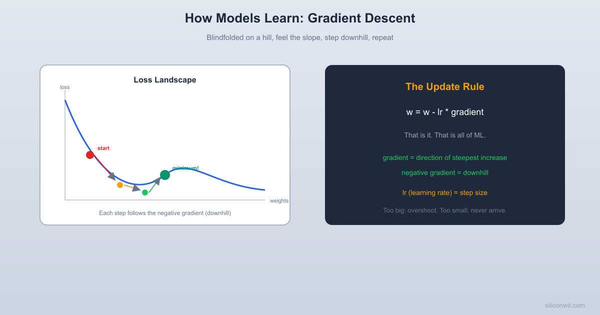
print("\nBottom-right: the contour plot shows the loss landscape.")
print("The GD path (red) starts at a random point and follows the")
print("gradient downhill to the minimum (black X).")