Complex Numbers and Phasors

Modified: Mar. 15, 2026

Published: Mar. 4, 2026

Become Contributor Expert Support

“Imaginary” is a terrible name. It was coined in the 17th century as an insult, and we have been stuck with it ever since. There is nothing imaginary about these numbers. They describe rotation. Once you see that, the mystery evaporates and one of the most powerful tools in engineering opens up. #ComplexNumbers #Phasors #Engineering

The Problem with “Imaginary”

The number (or in engineering, to avoid confusion with current) is defined by:

If you think of this as “the square root of negative one,” it sounds absurd. What number, multiplied by itself, gives a negative result? No real number does. That is why mathematicians called these numbers “imaginary” and moved on.

But here is a better way to think about it. Multiplying by is a 90-degree rotation. Start with the number 1 on the real number line. Multiply by and you get , which is one step up on the imaginary axis. Multiply by again and you get , which is back on the real axis but pointing the other direction. You have rotated 180 degrees in two steps of 90 degrees each.

           j (imaginary axis)
           |
           | j
           |
   -1 -----+------ 1    (real axis)
           |
           | -j
           |

Multiplying by rotates a number 90 degrees counterclockwise on this plane. That is all it does. That is why : two 90-degree rotations make a 180-degree rotation, which is the same as negation.

The Complex Plane

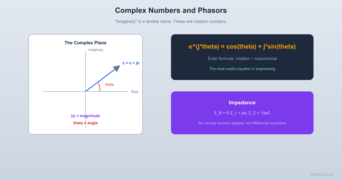
A complex number is a point in a 2D plane, where is the horizontal coordinate (real part) and is the vertical coordinate (imaginary part).

        Im
         |
    b ...+.........* z = a + jb
         |        /|
         |       / |
         |    r /  |
         |     /   |
         |    / θ  |
         |   /     |
    -----+--/------+------ Re
         |         a

The same point can be described in polar form:

where:

• is the magnitude (distance from the origin)
• is the phase angle

This should remind you of vectors. A complex number IS a 2D vector, just written in a notation that makes multiplication and rotation trivially easy.

Why Two Representations?

The rectangular form is best for addition. The polar form is best for multiplication.

Addition (rectangular):

Just add the components, exactly like vector addition.

Multiplication (polar):

Multiply the magnitudes, add the angles. Multiplication in the complex plane is rotation and scaling. This is the key insight that makes phasors work.

Euler’s Formula

The bridge between trigonometry and complex exponentials is Euler’s formula:

This single equation connects three seemingly different branches of mathematics: exponentials, trigonometry, and complex numbers. It is, arguably, the most important formula in engineering mathematics.

Why It Works (Intuition)

Consider the Taylor series for , , and :

If you substitute into the exponential series and group real and imaginary terms, you get exactly . The even powers of contribute to the cosine (they are real), and the odd powers contribute to the sine (they are imaginary). It is not magic. It is algebra.

Euler’s Identity

Setting gives the famous identity:

Five fundamental constants (, , , 1, 0) in one equation. Beautiful, but what matters for engineering is the practical consequence: sinusoidal signals can be represented as complex exponentials, and complex exponentials are far easier to work with.

Phasors: Sinusoids as Rotating Vectors

Here is the payoff. Consider a sinusoidal voltage:

Using Euler’s formula, we can write this as the real part of a complex exponential:

The factor is the same for all signals at the same frequency. So we strip it away and keep only the part that differs from signal to signal:

This is the phasor representation of the voltage. It captures the amplitude and the phase in a single complex number, dropping the time dependence because it is the same for everything.

        Im
         |
         |   * V_m e^(jφ)
         |  /
         | / V_m
         |/  φ
    -----+------------- Re
         |

    The phasor is a snapshot of the rotating vector.
    At any time t, the actual voltage is the real part
    of this vector after it has rotated by ωt more.

Why Phasors Are So Powerful

Without phasors, analyzing an AC circuit means solving differential equations. With phasors, the same analysis becomes algebra. Differentiation becomes multiplication by . Integration becomes division by . The entire calculus disappears, replaced by complex arithmetic.

Impedance: Resistance for AC Circuits

In DC circuits, Ohm’s law is . In AC circuits with phasors, the equivalent is:

where is the impedance, a complex number that generalizes resistance to include the effects of capacitors and inductors.

The Three Building Blocks

Combining Impedances

Impedances combine exactly like resistances:

• Series:
• Parallel:

Your phone charger converts AC from the wall outlet to DC for the battery. The efficiency of that conversion depends on impedance matching between the transformer windings, which is calculated using complex numbers. A mismatch means wasted power and heat.

Audio equalizers also rely on this math. When you boost the bass or cut the treble on your phone, the equalizer is adjusting the gain at different frequencies using complex transfer functions, exactly like the RC filter analysis below.

This is why phasors were invented. You can analyze any AC circuit using the same rules you learned for DC circuits, just with complex numbers instead of real ones.

Worked Example: RC Low-Pass Filter

Let us analyze the most common filter in electronics: the RC low-pass filter.

        R
  Vin o---/\/\/---+--- o Vout
                  |
                 === C
                  |
  GND o-----------+--- o GND

We want to find the ratio as a function of frequency.

Step 1: Write the Impedances

The resistor and capacitor are in series, forming a voltage divider. The output is taken across the capacitor.

Step 2: Voltage Divider

Multiply numerator and denominator by :

Step 3: Magnitude and Phase

The magnitude of the transfer function (gain) is:

The phase is:

Step 4: The Cutoff Frequency

The cutoff frequency is defined as the frequency where the output power drops to half (or the voltage drops to of the input):

This happens when , which gives:

For and :

Signals below 1592 Hz pass through mostly unchanged. Signals above 1592 Hz are attenuated. That is why it is called a low-pass filter.

Python: Complex Numbers and Phasors

Python has native support for complex numbers, and NumPy extends this to arrays.

import numpy as np
import matplotlib.pyplot as plt

# --- Complex number basics ---
z1 = 3 + 4j
z2 = 1 - 2j

print(f"z1 = {z1}")
print(f"z2 = {z2}")
print(f"z1 + z2 = {z1 + z2}")
print(f"z1 * z2 = {z1 * z2}")
print(f"|z1| = {abs(z1):.3f}")
print(f"angle(z1) = {np.angle(z1, deg=True):.1f} degrees")
print(f"Real part: {z1.real}, Imaginary part: {z1.imag}")

# --- Euler's formula verification ---
theta = np.pi / 4  # 45 degrees
euler = np.exp(1j * theta)
trig = np.cos(theta) + 1j * np.sin(theta)
print(f"\ne^(j*pi/4) = {euler:.4f}")
print(f"cos + j*sin = {trig:.4f}")
print(f"Difference: {abs(euler - trig):.2e}")

RC Filter Frequency Response

import numpy as np
import matplotlib.pyplot as plt

# Component values
R = 10e3      # 10 kohm
C = 10e-9     # 10 nF

# Cutoff frequency
f_c = 1 / (2 * np.pi * R * C)
print(f"Cutoff frequency: {f_c:.1f} Hz")

# Frequency sweep (logarithmic)
f = np.logspace(1, 6, 500)   # 10 Hz to 1 MHz
omega = 2 * np.pi * f

# Transfer function H(jw) = 1 / (1 + jwRC)
H = 1 / (1 + 1j * omega * R * C)

# Magnitude in dB and phase in degrees
magnitude_dB = 20 * np.log10(np.abs(H))
phase_deg = np.angle(H, deg=True)

# Bode plot
fig, (ax1, ax2) = plt.subplots(2, 1, figsize=(9, 7), sharex=True)

ax1.semilogx(f, magnitude_dB, 'b-', linewidth=2)
ax1.axhline(y=-3, color='r', linestyle='--', alpha=0.7, label='-3 dB')
ax1.axvline(x=f_c, color='gray', linestyle=':', alpha=0.7, label=f'fc = {f_c:.0f} Hz')
ax1.set_ylabel('Magnitude (dB)')
ax1.set_title('RC Low-Pass Filter Bode Plot')
ax1.legend()
ax1.grid(True, which='both', alpha=0.3)
ax1.set_ylim(-40, 5)

ax2.semilogx(f, phase_deg, 'b-', linewidth=2)
ax2.axhline(y=-45, color='r', linestyle='--', alpha=0.7, label='-45 deg at fc')
ax2.axvline(x=f_c, color='gray', linestyle=':', alpha=0.7)
ax2.set_ylabel('Phase (degrees)')
ax2.set_xlabel('Frequency (Hz)')
ax2.legend()
ax2.grid(True, which='both', alpha=0.3)
ax2.set_ylim(-100, 10)

plt.tight_layout()
plt.show()

Plotting Phasors

import numpy as np
import matplotlib.pyplot as plt

# Three phasors: voltage source, resistor voltage, capacitor voltage
# At the cutoff frequency (wRC = 1)
V_in = 1 + 0j                          # Reference: 1V at 0 degrees
H_c = 1 / (1 + 1j)                     # Capacitor voltage / V_in at wRC=1
V_C = V_in * H_c                       # Capacitor voltage phasor
V_R = V_in - V_C                       # Resistor voltage phasor

phasors = {'V_in': V_in, 'V_R': V_R, 'V_C': V_C}
colors = {'V_in': 'blue', 'V_R': 'red', 'V_C': 'green'}

fig, ax = plt.subplots(figsize=(7, 7))
for name, z in phasors.items():
    ax.annotate('', xy=(z.real, z.imag), xytext=(0, 0),
                arrowprops=dict(arrowstyle='->', color=colors[name], lw=2))
    ax.text(z.real * 1.1, z.imag * 1.1 + 0.03,
            f'{name} = {abs(z):.3f} at {np.angle(z, deg=True):.1f} deg',
            color=colors[name], fontsize=10)

ax.set_xlim(-0.2, 1.2)
ax.set_ylim(-0.8, 0.4)
ax.set_aspect('equal')
ax.grid(True, alpha=0.3)
ax.axhline(y=0, color='k', linewidth=0.5)
ax.axvline(x=0, color='k', linewidth=0.5)
ax.set_xlabel('Real')
ax.set_ylabel('Imaginary')
ax.set_title('Phasor Diagram at Cutoff Frequency (wRC = 1)')
plt.tight_layout()
plt.show()

Common Pitfalls

Summary

Complex numbers are not abstract curiosities. They are the natural language for describing anything that rotates or oscillates. Here is the chain of ideas:

1. Complex numbers are 2D numbers. They have a real part and an imaginary part, forming a point (or arrow) in the complex plane.

2. Multiplication is rotation and scaling. Multiplying by rotates by angle . Multiplying by scales by .

3. Euler’s formula connects exponentials and trigonometry. . This lets you represent sinusoidal signals as complex exponentials.

4. Phasors strip away time. A phasor captures the amplitude and phase of a sinusoidal signal, letting you analyze AC circuits with algebra instead of differential equations.

5. Impedance generalizes resistance. Resistors, inductors, and capacitors each have a complex impedance. Circuit analysis proceeds with the same rules as DC, just with complex arithmetic.

6. The cutoff frequency falls out naturally. For an RC filter, setting gives , the boundary between passed and attenuated frequencies.

In the next lesson on differential equations, you will see complex numbers appear again: the solutions to second-order ODEs involve complex exponentials, and the imaginary part of the eigenvalue gives the oscillation frequency while the real part gives the decay rate.