Monte Carlo Methods for Engineering Decisions

import numpy as np
import matplotlib.pyplot as plt

# ============================================================
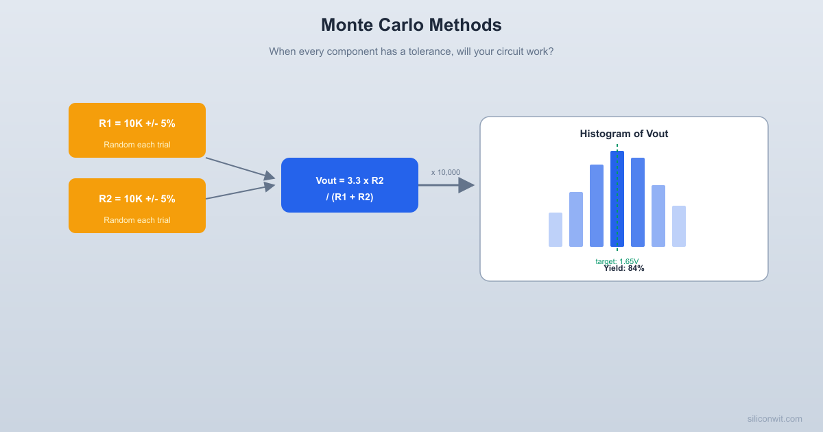
# Monte Carlo Tolerance Stackup Analyzer
# ============================================================
# Analyzes how component tolerances affect system performance
# and predicts manufacturing yield.

np.random.seed(42)

N_TRIALS = 50000  # Number of Monte Carlo trials

# ============================================================
# Example 1: Voltage Divider Tolerance Analysis
# ============================================================
# Circuit: Vin ---[R1]---+---[R2]--- GND
#                        |
#                       Vout
#
# Vout = Vin * R2 / (R1 + R2)
#
# Nominal design: Vin = 5.0V, R1 = 10k, R2 = 20k
# Target Vout = 5.0 * 20k / (10k + 20k) = 3.333 V
# Specification: 3.3 V +/- 0.1 V (3.2 to 3.4 V)

Vin_nominal = 5.0
R1_nominal = 10e3   # 10 kohm
R2_nominal = 20e3   # 20 kohm

Vout_target = Vin_nominal * R2_nominal / (R1_nominal + R2_nominal)
Vout_spec_low = 3.2
Vout_spec_high = 3.4

print("=" * 65)
print("  Monte Carlo Tolerance Stackup Analysis")
print("=" * 65)
print(f"  Voltage divider: Vin={Vin_nominal}V, R1={R1_nominal/1e3:.0f}k, R2={R2_nominal/1e3:.0f}k")
print(f"  Nominal Vout:    {Vout_target:.4f} V")
print(f"  Specification:   {Vout_spec_low:.1f} V to {Vout_spec_high:.1f} V")
print(f"  Trials:          {N_TRIALS:,}")
print("-" * 65)

def voltage_divider_mc(R1_nom, R2_nom, Vin, tolerance_pct, n_trials):
    """
    Run Monte Carlo simulation for a voltage divider.
    Components are assumed to have uniform distribution within tolerance.
    (Uniform is conservative; real resistors often follow truncated Gaussian.)
    """
    tol = tolerance_pct / 100.0

    # Sample R1 and R2 from uniform distribution within tolerance
    R1_samples = R1_nom * (1 + tol * (2 * np.random.rand(n_trials) - 1))
    R2_samples = R2_nom * (1 + tol * (2 * np.random.rand(n_trials) - 1))

    # Compute Vout for each trial
    Vout_samples = Vin * R2_samples / (R1_samples + R2_samples)

    return Vout_samples

# Run for different tolerance grades
tolerances = [1, 2, 5, 10]
results = {}

for tol in tolerances:
    vout = voltage_divider_mc(R1_nominal, R2_nominal, Vin_nominal, tol, N_TRIALS)

    in_spec = np.sum((vout >= Vout_spec_low) & (vout <= Vout_spec_high))
    yield_pct = 100.0 * in_spec / N_TRIALS

    results[tol] = {
        'vout': vout,
        'mean': np.mean(vout),
        'std': np.std(vout),
        'min': np.min(vout),
        'max': np.max(vout),
        'yield': yield_pct,
    }

    print(f"  {tol:2d}% tolerance: mean={np.mean(vout):.4f}V, "
          f"std={np.std(vout):.4f}V, "
          f"range=[{np.min(vout):.3f}, {np.max(vout):.3f}]V, "
          f"yield={yield_pct:.1f}%")

# ============================================================
# Example 2: Mechanical Tolerance Stackup
# ============================================================
# Assembly: shaft inserted into bearing, bearing pressed into housing
#
#   |<-- Housing bore -->|
#   |  |<-- Bearing OD ->|  |
#   |  |  |<- Bearing ID ->|  |
#   |  |  |  |<- Shaft OD ->|  |
#
# Clearance = Bearing_ID - Shaft_OD
# Interference = Bearing_OD - Housing_bore (press fit)
#
# We need: clearance > 0.01 mm (shaft must spin freely)
#          interference > 0.005 mm (bearing must not fall out)

print("\n" + "=" * 65)
print("  Mechanical Tolerance Stackup: Shaft + Bearing + Housing")
print("=" * 65)

# Nominal dimensions (mm)
shaft_od_nom = 25.000
bearing_id_nom = 25.030   # 30 um nominal clearance
bearing_od_nom = 47.000
housing_bore_nom = 46.985  # 15 um nominal interference

# Manufacturing tolerances (mm), assumed Gaussian (3-sigma = tolerance)
shaft_tol = 0.010      # +/- 10 um
bearing_id_tol = 0.008  # +/- 8 um
bearing_od_tol = 0.008  # +/- 8 um
housing_tol = 0.012     # +/- 12 um

# Sample dimensions (Gaussian, 3-sigma = tolerance)
shaft_od = np.random.normal(shaft_od_nom, shaft_tol / 3, N_TRIALS)
bearing_id = np.random.normal(bearing_id_nom, bearing_id_tol / 3, N_TRIALS)
bearing_od = np.random.normal(bearing_od_nom, bearing_od_tol / 3, N_TRIALS)
housing_bore = np.random.normal(housing_bore_nom, housing_tol / 3, N_TRIALS)

# Compute clearance and interference
clearance = bearing_id - shaft_od       # must be > 0.01 mm
interference = bearing_od - housing_bore  # must be > 0.005 mm

clearance_ok = clearance > 0.01
interference_ok = interference > 0.005
both_ok = clearance_ok & interference_ok

mech_yield = 100.0 * np.sum(both_ok) / N_TRIALS

print(f"  Shaft OD:       {shaft_od_nom:.3f} +/- {shaft_tol:.3f} mm")
print(f"  Bearing ID:     {bearing_id_nom:.3f} +/- {bearing_id_tol:.3f} mm")
print(f"  Bearing OD:     {bearing_od_nom:.3f} +/- {bearing_od_tol:.3f} mm")
print(f"  Housing bore:   {housing_bore_nom:.3f} +/- {housing_tol:.3f} mm")
print(f"  ---")
print(f"  Clearance:      mean={np.mean(clearance):.4f} mm, "
      f"std={np.std(clearance):.4f} mm")
print(f"  Interference:   mean={np.mean(interference):.4f} mm, "
      f"std={np.std(interference):.4f} mm")
print(f"  Clearance OK:   {100*np.mean(clearance_ok):.1f}%")
print(f"  Interference OK:{100*np.mean(interference_ok):.1f}%")
print(f"  Both OK (yield):{mech_yield:.1f}%")
print("=" * 65)

# ============================================================
# Sensitivity analysis: which component matters most?
# ============================================================
print("\n--- Sensitivity Analysis (Voltage Divider, 5% tolerance) ---")

# Baseline
baseline_std = results[5]['std']

# Tighten R1 only to 1%
vout_tight_r1 = voltage_divider_mc(R1_nominal, R2_nominal, Vin_nominal, 1, N_TRIALS)
# Keep R1 at 5%, measured as if R2 is tight
R1_5pct = R1_nominal * (1 + 0.05 * (2 * np.random.rand(N_TRIALS) - 1))
R2_1pct = R2_nominal * (1 + 0.01 * (2 * np.random.rand(N_TRIALS) - 1))
vout_tight_r2 = Vin_nominal * R2_1pct / (R1_5pct + R2_1pct)

# Tighten R2 only to 1%
R1_5pct2 = R1_nominal * (1 + 0.05 * (2 * np.random.rand(N_TRIALS) - 1))
R2_1pct2 = R2_nominal * (1 + 0.01 * (2 * np.random.rand(N_TRIALS) - 1))
vout_tight_r2_only = Vin_nominal * R2_1pct2 / (R1_5pct2 + R2_1pct2)

print(f"  Both at 5%:     std = {baseline_std:.5f} V")
print(f"  Both at 1%:     std = {np.std(vout_tight_r1):.5f} V")
print(f"  R1=5%, R2=1%:   std = {np.std(vout_tight_r2):.5f} V")
print(f"  R1=5%, R2=1%:   std = {np.std(vout_tight_r2_only):.5f} V")
print(f"  -> Tightening R2 alone reduces variation because R2 is larger")
print(f"     and contributes more to the output voltage sensitivity.")

# ============================================================
# Plot results
# ============================================================
fig, axes = plt.subplots(2, 2, figsize=(14, 10))

# Plot 1: Voltage divider histograms for each tolerance
ax = axes[0, 0]
colors = ['green', 'blue', 'orange', 'red']
for tol, color in zip(tolerances, colors):
    r = results[tol]
    ax.hist(r['vout'], bins=80, alpha=0.5, color=color, density=True,
            label=f'{tol}% tol (yield={r["yield"]:.1f}%)')
ax.axvline(Vout_spec_low, color='black', linestyle='--', linewidth=2, label='Spec limits')
ax.axvline(Vout_spec_high, color='black', linestyle='--', linewidth=2)
ax.axvline(Vout_target, color='black', linestyle='-', linewidth=1, alpha=0.5)
ax.set_xlabel('Output Voltage (V)')
ax.set_ylabel('Probability Density')
ax.set_title('Voltage Divider: Output Distribution by Tolerance Grade')
ax.legend(fontsize=8)
ax.grid(True, alpha=0.3)

# Plot 2: Yield vs tolerance
ax = axes[0, 1]
yields = [results[t]['yield'] for t in tolerances]
ax.bar([str(t) + '%' for t in tolerances], yields, color=colors, alpha=0.7,
       edgecolor='black')
ax.axhline(y=99.0, color='green', linestyle='--', alpha=0.7, label='99% target')
ax.axhline(y=95.0, color='orange', linestyle='--', alpha=0.7, label='95% target')
ax.set_xlabel('Component Tolerance')
ax.set_ylabel('Yield (%)')
ax.set_title('Manufacturing Yield vs Component Tolerance')
ax.legend()
ax.grid(True, alpha=0.3, axis='y')
for i, (tol, y) in enumerate(zip(tolerances, yields)):
    ax.text(i, y + 0.5, f'{y:.1f}%', ha='center', fontsize=10, fontweight='bold')

# Plot 3: Mechanical clearance histogram
ax = axes[1, 0]
ax.hist(clearance * 1000, bins=80, alpha=0.6, color='steelblue', density=True,
        label=f'Clearance (yield={100*np.mean(clearance_ok):.1f}%)')
ax.axvline(10, color='red', linestyle='--', linewidth=2, label='Min clearance (10 um)')
ax.axvline(0, color='black', linestyle='-', linewidth=1, alpha=0.5)
ax.set_xlabel('Clearance (um)')
ax.set_ylabel('Probability Density')
ax.set_title('Shaft-Bearing Clearance Distribution')
ax.legend(fontsize=9)
ax.grid(True, alpha=0.3)

# Plot 4: Mechanical interference histogram
ax = axes[1, 1]
ax.hist(interference * 1000, bins=80, alpha=0.6, color='coral', density=True,
        label=f'Interference (yield={100*np.mean(interference_ok):.1f}%)')
ax.axvline(5, color='red', linestyle='--', linewidth=2, label='Min interference (5 um)')
ax.axvline(0, color='black', linestyle='-', linewidth=1, alpha=0.5)
ax.set_xlabel('Interference (um)')
ax.set_ylabel('Probability Density')
ax.set_title('Bearing-Housing Interference Distribution')
ax.legend(fontsize=9)
ax.grid(True, alpha=0.3)

plt.tight_layout()
plt.savefig('monte_carlo_tolerance.png', dpi=150, bbox_inches='tight')
plt.show()
print("\nPlot saved: monte_carlo_tolerance.png")

References

• Gilks, W. R. et al. (1995). Markov Chain Monte Carlo in Practice. Chapman and Hall. The statistical foundations.
• Bruns, M. (2006). Tolerance Analysis and Optimization of Mechanical Assemblies. PhD Thesis, University of Erlangen. Good coverage of mechanical tolerance stackup methods.
• Hayter, A. J. (2012). Probability and Statistics for Engineers and Scientists. Cengage. Covers the statistical fundamentals behind Monte Carlo.
• Analog Devices Application Note AN-1208. Component Tolerances and their Effect on Filter Performance. Practical tolerance analysis for analog circuits.
Comments
Loading comments...
© 2021-2026 SiliconWit®. All rights reserved.