Fourier Analysis and the Frequency Domain

Modified: Mar. 15, 2026

Published: Mar. 7, 2026

Become Contributor Expert Support

A vibrating guitar string does not produce a single pure tone. It produces a fundamental frequency plus harmonics: integer multiples of the fundamental that give the note its character. A noisy sensor signal is a slow, meaningful change buried under fast, random fluctuations. A digital communication signal is multiple frequencies carefully packed together. In every case, the signal is a sum of sine waves at different frequencies. Fourier analysis is the mathematical tool that decomposes any signal into those individual frequency components. #Fourier #FrequencyDomain #SignalProcessing

The Big Idea: Any Signal Is a Sum of Sines

Joseph Fourier’s insight, radical when he proposed it in 1807, was that any periodic signal can be written as a sum of sines and cosines:

where is the fundamental frequency and the coefficients , tell you how much of each frequency is present.

This is not an approximation. Given enough terms, the sum converges exactly to the original signal. A square wave, a sawtooth, a triangle wave, even a single sharp spike: all can be built from smooth sine waves if you use enough of them.

Original signal (square wave):
     ___________
    |           |
    |           |
____|           |____________

= Sum of odd harmonics:

~  sin(t)       (fundamental)
+  sin(3t)/3    (3rd harmonic)
+  sin(5t)/5    (5th harmonic)
+  sin(7t)/7    (7th harmonic)
+  ...

More terms = sharper corners

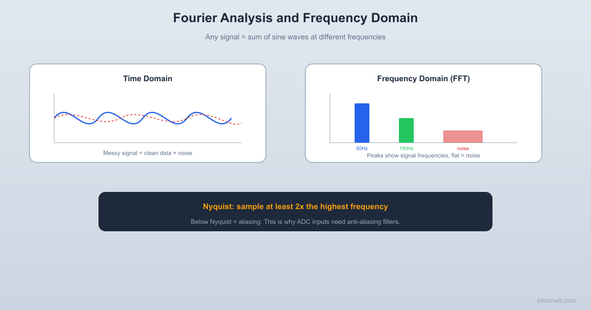
Time Domain vs. Frequency Domain

These are two ways of looking at the same signal. The time domain shows amplitude versus time: what you see on an oscilloscope. The frequency domain shows amplitude versus frequency: what you see on a spectrum analyzer. Neither view contains more information than the other. They are equivalent representations.

Why Frequency Matters for Engineers

A temperature sensor reading has two components:

• Low-frequency: the actual temperature, changing slowly over minutes
• High-frequency: electrical noise, changing rapidly over microseconds

In the time domain, these are mixed together. In the frequency domain, they are separated. A low-pass filter that keeps low frequencies and blocks high frequencies extracts the real signal from the noise. You cannot design this filter without thinking in the frequency domain.

The Discrete Fourier Transform (DFT) and FFT

Real signals are sampled at discrete times. The DFT takes time-domain samples and produces frequency-domain coefficients:

Each is a complex number whose magnitude tells you the amplitude at frequency and whose phase tells you the time shift.

The Fast Fourier Transform (FFT) computes the same result as the DFT but in operations instead of . For samples, the FFT is about 100 times faster than the direct computation. This is what makes real-time spectral analysis possible on microcontrollers.

You do not need to understand the FFT algorithm (the Cooley-Tukey butterfly diagram) to use it effectively. What matters is understanding what goes in and what comes out.

What the FFT Output Means

Given samples taken at sampling rate :

• The FFT produces complex values
• Frequencies range from to , but only the first are unique (the rest are mirror images)
• The frequency resolution is
• To resolve two close frequencies, you need a longer recording (more samples at the same rate)

Python: Building a Signal and Finding Its Frequencies

import numpy as np
import matplotlib.pyplot as plt

# Create a signal: 50 Hz + 120 Hz + noise
fs = 1000  # sampling rate (Hz)
duration = 0.5  # seconds
t = np.arange(0, duration, 1/fs)
N = len(t)

# Clean signal components
signal = 1.0 * np.sin(2 * np.pi * 50 * t) + \
         0.5 * np.sin(2 * np.pi * 120 * t)

# Add noise
np.random.seed(42)
noisy_signal = signal + 0.8 * np.random.randn(N)

# Compute FFT
fft_vals = np.fft.fft(noisy_signal)
freqs = np.fft.fftfreq(N, 1/fs)

# Take only positive frequencies and compute magnitude
pos_mask = freqs >= 0
freqs_pos = freqs[pos_mask]
magnitude = 2.0 / N * np.abs(fft_vals[pos_mask])

# Plot
fig, (ax1, ax2) = plt.subplots(2, 1, figsize=(10, 6))

ax1.plot(t * 1000, noisy_signal, 'b-', linewidth=0.5)
ax1.set_xlabel('Time (ms)')
ax1.set_ylabel('Amplitude')
ax1.set_title('Time Domain: Noisy Signal')
ax1.set_xlim(0, 100)  # show first 100 ms
ax1.grid(True, alpha=0.3)

ax2.plot(freqs_pos, magnitude, 'r-', linewidth=1)
ax2.set_xlabel('Frequency (Hz)')
ax2.set_ylabel('Magnitude')
ax2.set_title('Frequency Domain: FFT Spectrum')
ax2.set_xlim(0, 250)
ax2.grid(True, alpha=0.3)

# Mark the peaks
ax2.annotate('50 Hz', xy=(50, magnitude[np.argmin(np.abs(freqs_pos - 50))]),
             fontsize=10, ha='center', va='bottom')
ax2.annotate('120 Hz', xy=(120, magnitude[np.argmin(np.abs(freqs_pos - 120))]),
             fontsize=10, ha='center', va='bottom')

plt.tight_layout()
plt.show()

The noisy time-domain signal looks like a mess. The frequency-domain plot clearly shows two spikes at 50 Hz and 120 Hz, exactly the frequencies we put in. The noise, spread across all frequencies, appears as a low baseline. This is the power of Fourier analysis: it reveals structure hidden in noise.

The Sampling Theorem (Nyquist)

How fast do you need to sample a signal? The Nyquist-Shannon sampling theorem gives the answer: you must sample at least twice the highest frequency present in the signal.

If your signal contains frequencies up to 100 Hz, you need at least 200 samples per second. If you sample slower than this, you get aliasing: high frequencies masquerade as low frequencies, and no amount of post-processing can fix it.

Aliasing: What Goes Wrong

Imagine a wheel spinning at 9 revolutions per second, filmed at 10 frames per second. The wheel appears to spin at 1 revolution per second. That is aliasing: undersampling causes a high frequency to appear as a lower frequency.

True signal: 90 Hz sine wave
Sampled at:  100 Hz (barely above Nyquist)

What you reconstruct: 10 Hz sine wave (alias!)

The samples land at the same points for both
the 90 Hz and 10 Hz signals:

90 Hz:  /\/\/\/\/\/\/\/\/\/\  (fast oscillation)
        *     *     *     *   (samples every 10 ms)

10 Hz:  /          \          (slow oscillation)
        *     *     *     *   (same sample values!)

The alias frequency is where is the nearest integer multiple of .

Python: Demonstrating Aliasing

import numpy as np
import matplotlib.pyplot as plt

# True signal: 90 Hz
f_true = 90  # Hz
t_fine = np.linspace(0, 0.1, 10000)  # "continuous" signal
signal_true = np.sin(2 * np.pi * f_true * t_fine)

# Sample at different rates
fig, axes = plt.subplots(3, 1, figsize=(10, 8))
sample_rates = [500, 200, 100]
titles = [
    f'fs=500 Hz (well above Nyquist)',
    f'fs=200 Hz (above Nyquist)',
    f'fs=100 Hz (below Nyquist: aliasing!)'
]

for ax, fs, title in zip(axes, sample_rates, titles):
    t_sampled = np.arange(0, 0.1, 1/fs)
    sampled = np.sin(2 * np.pi * f_true * t_sampled)

    ax.plot(t_fine * 1000, signal_true, 'b-', alpha=0.3,
            linewidth=1, label=f'True {f_true} Hz')
    ax.plot(t_sampled * 1000, sampled, 'ro-', markersize=5,
            label=f'Sampled at {fs} Hz')

    # Show reconstructed (aliased) signal
    if fs < 2 * f_true:
        f_alias = abs(f_true - fs)
        alias_signal = np.sin(2 * np.pi * f_alias * t_fine)
        ax.plot(t_fine * 1000, alias_signal, 'g--', linewidth=2,
                label=f'Alias: {f_alias} Hz')

    ax.set_title(title)
    ax.set_ylabel('Amplitude')
    ax.legend(fontsize=8, loc='upper right')
    ax.grid(True, alpha=0.3)
    ax.set_xlim(0, 50)

axes[2].set_xlabel('Time (ms)')
plt.tight_layout()
plt.show()

Anti-Aliasing Filters

Since aliasing is irreversible once the signal is digitized, you must prevent it before sampling. An anti-aliasing filter is an analog low-pass filter placed before the ADC that removes all frequencies above .

Every properly designed data acquisition system has one. Without it, a high-frequency spike from a motor, a radio transmitter, or mains interference could alias into your measurement band and corrupt your data. You would see a slow oscillation in your data that does not physically exist.

This is why the sampling rate and the anti-aliasing filter must be designed together. If your ADC samples at 1 kHz, you need a low-pass filter with a cutoff well below 500 Hz. In practice, you oversample (use a higher sample rate than strictly necessary) so the filter does not need to be extremely sharp.

Spectral Analysis Applications

Python: Spectral Analysis of a Vibration Signal

import numpy as np
import matplotlib.pyplot as plt

# Simulate vibration from a machine
# Shaft at 30 Hz, bearing defect at 127 Hz, structural resonance at 250 Hz
fs = 2000  # sample rate (Hz)
duration = 2.0
t = np.arange(0, duration, 1/fs)
N = len(t)

np.random.seed(42)
vibration = (1.0 * np.sin(2 * np.pi * 30 * t) +      # shaft
             0.3 * np.sin(2 * np.pi * 127 * t) +      # bearing
             0.15 * np.sin(2 * np.pi * 250 * t) +     # resonance
             0.2 * np.random.randn(N))                  # background noise

# Compute FFT
fft_vals = np.fft.fft(vibration)
freqs = np.fft.fftfreq(N, 1/fs)
pos_mask = freqs >= 0
freqs_pos = freqs[pos_mask]
magnitude = 2.0 / N * np.abs(fft_vals[pos_mask])

fig, (ax1, ax2) = plt.subplots(2, 1, figsize=(10, 6))

ax1.plot(t[:500] * 1000, vibration[:500], 'b-', linewidth=0.8)
ax1.set_xlabel('Time (ms)')
ax1.set_ylabel('Acceleration (g)')
ax1.set_title('Vibration Signal (Time Domain)')
ax1.grid(True, alpha=0.3)

ax2.plot(freqs_pos, magnitude, 'r-', linewidth=0.8)
ax2.set_xlabel('Frequency (Hz)')
ax2.set_ylabel('Magnitude')
ax2.set_title('Vibration Spectrum (Frequency Domain)')
ax2.set_xlim(0, 400)
ax2.grid(True, alpha=0.3)

# Annotate peaks
for f_peak, label in [(30, 'Shaft\n30 Hz'), (127, 'Bearing\n127 Hz'),
                       (250, 'Resonance\n250 Hz')]:
    idx = np.argmin(np.abs(freqs_pos - f_peak))
    ax2.annotate(label, xy=(f_peak, magnitude[idx]),
                 xytext=(f_peak, magnitude[idx] + 0.15),
                 ha='center', fontsize=9,
                 arrowprops=dict(arrowstyle='->', color='black'))

plt.tight_layout()
plt.show()

Windowing: Reducing Spectral Leakage

The FFT assumes your signal is periodic with period equal to your recording length. If it is not (and it usually is not), the discontinuity at the edges creates spurious frequency content called spectral leakage. The spectrum shows broad skirts around each peak instead of sharp spikes.

A window function tapers the signal to zero at both ends, reducing the discontinuity. Common windows:

• Hanning (Hann): good general-purpose choice
• Hamming: slightly less sidelobe suppression but narrower main lobe
• Blackman: excellent sidelobe suppression, wider main lobe
• Rectangular (no window): narrowest main lobe, worst leakage

import numpy as np
import matplotlib.pyplot as plt

# Signal with a frequency that doesn't fit exactly in the FFT length
fs = 1000
N = 256
t = np.arange(N) / fs
f_signal = 47.3  # Hz (not a bin center for N=256, fs=1000)

signal = np.sin(2 * np.pi * f_signal * t)

# Apply different windows
windows = {
    'Rectangular (no window)': np.ones(N),
    'Hanning': np.hanning(N),
    'Blackman': np.blackman(N),
}

fig, axes = plt.subplots(len(windows), 1, figsize=(10, 8))
for ax, (name, w) in zip(axes, windows.items()):
    windowed = signal * w
    fft_mag = 2.0 / np.sum(w) * np.abs(np.fft.fft(windowed))
    freqs = np.fft.fftfreq(N, 1/fs)

    pos = freqs >= 0
    ax.plot(freqs[pos], 20 * np.log10(fft_mag[pos] + 1e-10), linewidth=1)
    ax.set_title(name)
    ax.set_ylabel('Magnitude (dB)')
    ax.set_xlim(0, 150)
    ax.set_ylim(-60, 10)
    ax.grid(True, alpha=0.3)

axes[-1].set_xlabel('Frequency (Hz)')
plt.suptitle(f'Spectral Leakage: {f_signal} Hz signal', fontsize=12)
plt.tight_layout()
plt.show()

Key Relationships to Remember

Exercises

1. Build and decompose. Create a signal from three sine waves at 10 Hz, 25 Hz, and 60 Hz with amplitudes 1.0, 0.5, and 0.3. Add Gaussian noise. Compute the FFT and verify that the three peaks appear at the correct frequencies with approximately correct amplitudes.

2. Sampling rate experiment. Take a 100 Hz signal and sample it at 300 Hz, 200 Hz, 150 Hz, and 90 Hz. For each rate, compute the FFT. At which sampling rates does aliasing occur? What alias frequency do you observe?

3. Frequency resolution. Record (or simulate) a signal containing two close frequencies: 50 Hz and 52 Hz. How many seconds of data do you need to resolve them as separate peaks in the FFT?

4. Window comparison. Take a signal with a single frequency that does not fall on an FFT bin center. Apply rectangular, Hanning, and Blackman windows. Compare the spectral leakage. Which window would you choose for (a) detecting a weak signal near a strong one, (b) accurately measuring the frequency of a single tone?

5. Real signal analysis. Record audio from your phone’s microphone (a whistle, a tuning fork, or a musical note). Load the WAV file into Python, compute the FFT, and identify the fundamental frequency and harmonics.

References

• Smith, S. W. (1997). The Scientist and Engineer’s Guide to Digital Signal Processing. Free online: dspguide.com. Chapters 8-12 cover the DFT and FFT beautifully.
• Oppenheim, A. V. and Willsky, A. S. (1996). Signals and Systems. Prentice Hall.
• 3Blue1Brown. But what is the Fourier Transform? A visual introduction. youtube.com/watch?v=spUNpyF58BY