Control System Design in Simulation

              error        PID         voltage       DC Motor       speed
 setpoint -->(+)--------> [Kp,Ki,Kd] ---------> [ Motor Model ] --------+---> output
              ^  -                                                       |
              |                                                          |
              +----------------------------------------------------------+
                                  feedback (measured speed)

"""
PID Motor Controller Simulator
Models a DC motor with PID speed control.
Includes auto-tuning via grid search.
"""

import numpy as np
from scipy.integrate import solve_ivp
import matplotlib.pyplot as plt

# -------------------------------------------------------
# DC Motor parameters (small brushed motor, e.g., 12V hobby motor)
# -------------------------------------------------------
MOTOR = {
    "R": 0.5,          # Armature resistance (ohm)
    "L": 0.001,        # Armature inductance (H)
    "Kt": 0.02,        # Torque constant (N*m/A)
    "Ke": 0.02,        # Back-EMF constant (V*s/rad) = Kt in SI
    "J": 0.0005,       # Rotor inertia (kg*m^2)
    "b": 0.001,        # Viscous friction (N*m*s/rad)
    "V_max": 12.0,     # Maximum voltage (V)
}

# Target speed
SETPOINT_RPM = 1000.0
SETPOINT_RAD_S = SETPOINT_RPM * 2 * np.pi / 60.0

def rpm_to_rads(rpm):
    return rpm * 2 * np.pi / 60.0

def rads_to_rpm(rads):
    return rads * 60.0 / (2 * np.pi)

# -------------------------------------------------------
# PID Controller class
# -------------------------------------------------------
class PIDController:
    """PID controller with anti-windup."""

    def __init__(self, Kp, Ki, Kd, output_min=0.0, output_max=12.0,
                 integral_limit=50.0):
        self.Kp = Kp
        self.Ki = Ki
        self.Kd = Kd
        self.output_min = output_min
        self.output_max = output_max
        self.integral_limit = integral_limit

        self.integral = 0.0
        self.prev_error = 0.0
        self.prev_time = None

    def reset(self):
        self.integral = 0.0
        self.prev_error = 0.0
        self.prev_time = None

    def compute(self, error, t):
        if self.prev_time is None:
            dt = 0.001  # First call
        else:
            dt = t - self.prev_time
            if dt <= 0:
                dt = 0.001

        # Proportional
        P = self.Kp * error

        # Integral with anti-windup
        self.integral += error * dt
        self.integral = np.clip(self.integral,
                                 -self.integral_limit,
                                 self.integral_limit)
        I = self.Ki * self.integral

        # Derivative
        derivative = (error - self.prev_error) / dt
        D = self.Kd * derivative

        # Output with saturation
        output = P + I + D
        output = np.clip(output, self.output_min, self.output_max)

        self.prev_error = error
        self.prev_time = t

        return output

# -------------------------------------------------------
# Motor + PID simulation
# -------------------------------------------------------
def simulate_motor_pid(Kp, Ki, Kd, setpoint_rpm=1000.0, t_end=0.5,
                        n_points=2000, disturbance_time=None,
                        disturbance_torque=0.0):
    """
    Simulate a DC motor with PID speed control.
    Returns time, speed (RPM), current (A), voltage (V), error (RPM).
    """
    m = MOTOR
    setpoint_rads = rpm_to_rads(setpoint_rpm)

    pid = PIDController(Kp, Ki, Kd, output_min=0.0,
                         output_max=m["V_max"])

    # We cannot use solve_ivp directly with the PID controller
    # because the PID has internal state (integral, derivative).
    # Instead, we use a simple fixed-step Euler integration,
    # which also matches how PID runs on a microcontroller.

    dt = t_end / n_points
    t_arr = np.linspace(0, t_end, n_points)

    i_arr = np.zeros(n_points)    # Current
    w_arr = np.zeros(n_points)    # Angular velocity (rad/s)
    v_arr = np.zeros(n_points)    # Applied voltage
    e_arr = np.zeros(n_points)    # Error (rad/s)

    i = 0.0   # Initial current
    w = 0.0   # Initial speed

    for k in range(n_points):
        t = t_arr[k]

        # Error
        error = setpoint_rads - w
        e_arr[k] = rads_to_rpm(error)

        # PID controller
        voltage = pid.compute(error, t)
        v_arr[k] = voltage

        # External disturbance torque
        T_dist = 0.0
        if disturbance_time is not None and t >= disturbance_time:
            T_dist = disturbance_torque

        # Motor electrical dynamics: di/dt = (V - R*i - Ke*w) / L
        di_dt = (voltage - m["R"] * i - m["Ke"] * w) / m["L"]

        # Motor mechanical dynamics: dw/dt = (Kt*i - b*w + T_dist) / J
        dw_dt = (m["Kt"] * i - m["b"] * w - T_dist) / m["J"]

        # Store current state
        i_arr[k] = i
        w_arr[k] = rads_to_rpm(w)

        # Euler step
        i += di_dt * dt
        w += dw_dt * dt

        # Physical constraints
        i = max(i, 0)  # Current cannot be negative (no regenerative braking)
        w = max(w, 0)  # Speed cannot be negative

    return t_arr, w_arr, i_arr, v_arr, e_arr

# -------------------------------------------------------
# Step response metrics
# -------------------------------------------------------
def analyze_response(t, speed_rpm, setpoint_rpm):
    """
    Compute overshoot, settling time, rise time, and
    steady-state error from a step response.
    """
    sp = setpoint_rpm

    # Overshoot
    peak = np.max(speed_rpm)
    if peak > sp:
        overshoot_pct = (peak - sp) / sp * 100
    else:
        overshoot_pct = 0.0

    # Rise time (10% to 90% of setpoint)
    idx_10 = np.where(speed_rpm >= 0.1 * sp)[0]
    idx_90 = np.where(speed_rpm >= 0.9 * sp)[0]
    if len(idx_10) > 0 and len(idx_90) > 0:
        rise_time = t[idx_90[0]] - t[idx_10[0]]
    else:
        rise_time = float('inf')

    # Settling time (2% band)
    band = 0.02 * sp
    settled = np.abs(speed_rpm - sp) < band
    not_settled = np.where(~settled)[0]
    if len(not_settled) == 0:
        settling_time = 0.0
    else:
        last = not_settled[-1]
        settling_time = t[last] if last < len(t) - 1 else t[-1]

    # Steady-state error (average of last 10% of data)
    n_last = max(1, len(speed_rpm) // 10)
    ss_speed = np.mean(speed_rpm[-n_last:])
    ss_error = sp - ss_speed

    return {
        "overshoot_pct": overshoot_pct,
        "rise_time_ms": rise_time * 1000,
        "settling_time_ms": settling_time * 1000,
        "ss_error_rpm": ss_error,
        "peak_rpm": peak,
    }

# -------------------------------------------------------
# 1. Demonstrate P, PI, and PID
# -------------------------------------------------------
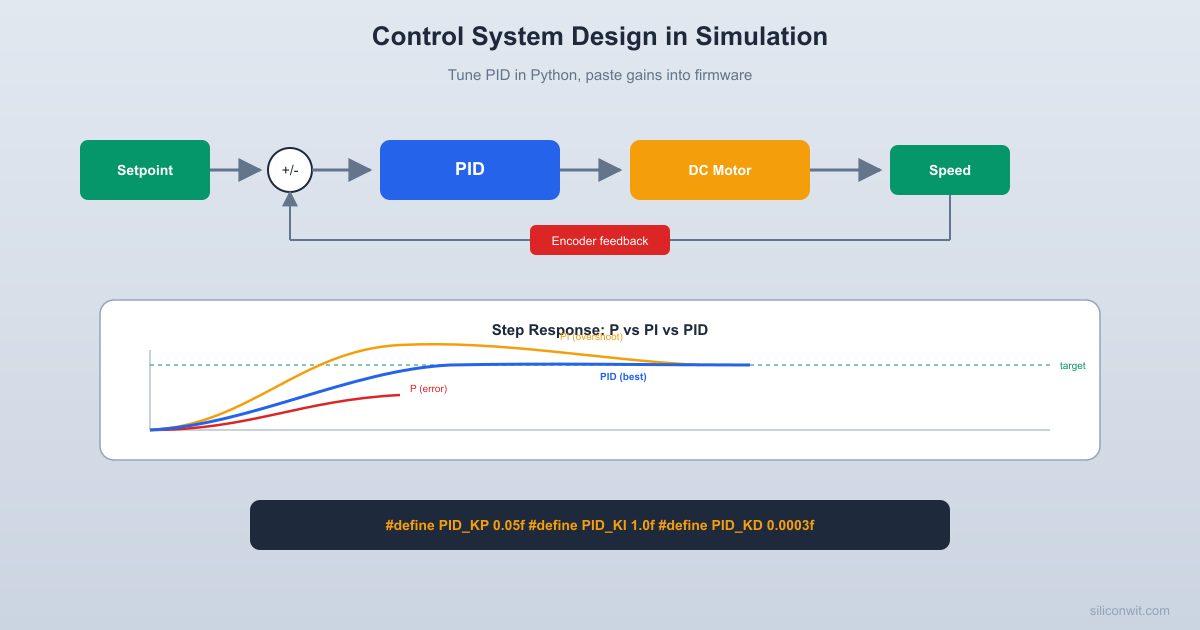
def demo_controller_types():
    """Show the effect of P, PI, and PID control."""

    configs = [
        ("P only (Kp=0.1)",         0.1, 0.0, 0.0),
        ("PI (Kp=0.1, Ki=2.0)",     0.1, 2.0, 0.0),
        ("PID (Kp=0.1, Ki=2.0, Kd=0.0005)", 0.1, 2.0, 0.0005),
    ]

    fig, axes = plt.subplots(2, 2, figsize=(13, 8))
    fig.suptitle("PID Motor Control: Controller Comparison",
                 fontsize=13, fontweight="bold")

    colors = ["tab:red", "tab:blue", "tab:green"]

    for (label, Kp, Ki, Kd), color in zip(configs, colors):
        t, speed, current, voltage, error = simulate_motor_pid(
            Kp, Ki, Kd, setpoint_rpm=SETPOINT_RPM, t_end=0.5)

        metrics = analyze_response(t, speed, SETPOINT_RPM)

        print(f"\n  {label}")
        print(f"    Overshoot:      {metrics['overshoot_pct']:.1f}%")
        print(f"    Rise time:      {metrics['rise_time_ms']:.1f} ms")
        print(f"    Settling time:  {metrics['settling_time_ms']:.1f} ms")
        print(f"    SS error:       {metrics['ss_error_rpm']:.1f} RPM")

        axes[0, 0].plot(t * 1000, speed, color=color, linewidth=2,
                         label=label)
        axes[0, 1].plot(t * 1000, current, color=color, linewidth=1.5,
                         label=label)
        axes[1, 0].plot(t * 1000, voltage, color=color, linewidth=1.5,
                         label=label)
        axes[1, 1].plot(t * 1000, error, color=color, linewidth=1.5,
                         label=label)

    # Format plots
    axes[0, 0].axhline(y=SETPOINT_RPM, color="gray", linestyle="--",
                        alpha=0.5, label="Setpoint")
    axes[0, 0].set_ylabel("Speed (RPM)")
    axes[0, 0].set_title("Motor Speed")
    axes[0, 0].legend(fontsize=7)
    axes[0, 0].grid(True, alpha=0.3)

    axes[0, 1].set_ylabel("Current (A)")
    axes[0, 1].set_title("Motor Current")
    axes[0, 1].legend(fontsize=7)
    axes[0, 1].grid(True, alpha=0.3)

    axes[1, 0].set_xlabel("Time (ms)")
    axes[1, 0].set_ylabel("Voltage (V)")
    axes[1, 0].set_title("Applied Voltage")
    axes[1, 0].legend(fontsize=7)
    axes[1, 0].grid(True, alpha=0.3)

    axes[1, 1].set_xlabel("Time (ms)")
    axes[1, 1].set_ylabel("Error (RPM)")
    axes[1, 1].set_title("Speed Error")
    axes[1, 1].legend(fontsize=7)
    axes[1, 1].grid(True, alpha=0.3)

    plt.tight_layout()
    plt.savefig("pid_comparison.png", dpi=150, bbox_inches="tight")
    plt.show()
    print("\nSaved: pid_comparison.png")

# -------------------------------------------------------
# 2. Sweep Kp to show its effect
# -------------------------------------------------------
def sweep_kp():
    """Sweep proportional gain and show the tradeoff."""

    kp_values = [0.02, 0.05, 0.1, 0.2, 0.5]
    Ki_fixed = 1.0
    Kd_fixed = 0.0003

    fig, axes = plt.subplots(1, 2, figsize=(13, 5))
    fig.suptitle("Effect of Proportional Gain (Kp)",
                 fontsize=13, fontweight="bold")

    colors = plt.cm.viridis(np.linspace(0.1, 0.9, len(kp_values)))

    overshoots = []
    settling_times = []

    for Kp, color in zip(kp_values, colors):
        t, speed, _, _, _ = simulate_motor_pid(
            Kp, Ki_fixed, Kd_fixed, t_end=0.5)
        metrics = analyze_response(t, speed, SETPOINT_RPM)
        overshoots.append(metrics["overshoot_pct"])
        settling_times.append(metrics["settling_time_ms"])

        axes[0].plot(t * 1000, speed, color=color, linewidth=2,
                     label=f"Kp={Kp}")

    axes[0].axhline(y=SETPOINT_RPM, color="gray", linestyle="--", alpha=0.5)
    axes[0].set_xlabel("Time (ms)")
    axes[0].set_ylabel("Speed (RPM)")
    axes[0].set_title("Step Response")
    axes[0].legend(fontsize=8)
    axes[0].grid(True, alpha=0.3)

    ax_os = axes[1]
    ax_st = ax_os.twinx()
    ax_os.plot(kp_values, overshoots, "o-", color="tab:red",
               linewidth=2, label="Overshoot (%)")
    ax_st.plot(kp_values, settling_times, "s-", color="tab:blue",
               linewidth=2, label="Settling time (ms)")
    ax_os.set_xlabel("Kp")
    ax_os.set_ylabel("Overshoot (%)", color="tab:red")
    ax_st.set_ylabel("Settling Time (ms)", color="tab:blue")
    axes[1].set_title("Kp Tradeoff")
    lines1, labels1 = ax_os.get_legend_handles_labels()
    lines2, labels2 = ax_st.get_legend_handles_labels()
    ax_os.legend(lines1 + lines2, labels1 + labels2, fontsize=8)
    ax_os.grid(True, alpha=0.3)

    plt.tight_layout()
    plt.savefig("kp_sweep.png", dpi=150, bbox_inches="tight")
    plt.show()
    print("Saved: kp_sweep.png")

# -------------------------------------------------------
# 3. Auto-tuner: grid search for optimal PID gains
# -------------------------------------------------------
def auto_tune():
    """
    Search for PID gains that minimize a cost function
    balancing settling time and overshoot.
    """
    print("\n" + "=" * 55)
    print("  PID AUTO-TUNER (Grid Search)")
    print("=" * 55)

    # Search space
    Kp_range = np.linspace(0.05, 0.3, 10)
    Ki_range = np.linspace(0.5, 5.0, 10)
    Kd_range = np.linspace(0.0001, 0.002, 8)

    total = len(Kp_range) * len(Ki_range) * len(Kd_range)
    print(f"  Evaluating {total} gain combinations...")

    best_cost = float('inf')
    best_gains = (0, 0, 0)
    best_metrics = None

    count = 0
    for Kp in Kp_range:
        for Ki in Ki_range:
            for Kd in Kd_range:
                count += 1

                t, speed, _, _, _ = simulate_motor_pid(
                    Kp, Ki, Kd, t_end=0.5, n_points=1000)
                metrics = analyze_response(t, speed, SETPOINT_RPM)

                # Cost function: weighted sum of settling time,
                # overshoot, and steady-state error
                cost = (metrics["settling_time_ms"] * 1.0 +
                        metrics["overshoot_pct"] * 5.0 +
                        abs(metrics["ss_error_rpm"]) * 0.5)

                # Penalize instability (very large overshoot)
                if metrics["overshoot_pct"] > 30:
                    cost += 1000

                if cost < best_cost:
                    best_cost = cost
                    best_gains = (Kp, Ki, Kd)
                    best_metrics = metrics

    Kp_opt, Ki_opt, Kd_opt = best_gains

    print(f"\n  Optimal gains found:")
    print(f"    Kp = {Kp_opt:.4f}")
    print(f"    Ki = {Ki_opt:.4f}")
    print(f"    Kd = {Kd_opt:.6f}")
    print(f"\n  Performance:")
    print(f"    Overshoot:      {best_metrics['overshoot_pct']:.1f}%")
    print(f"    Rise time:      {best_metrics['rise_time_ms']:.1f} ms")
    print(f"    Settling time:  {best_metrics['settling_time_ms']:.1f} ms")
    print(f"    SS error:       {best_metrics['ss_error_rpm']:.1f} RPM")
    print("=" * 55)

    # Simulate with optimal gains
    t, speed, current, voltage, error = simulate_motor_pid(
        Kp_opt, Ki_opt, Kd_opt, t_end=0.5, n_points=2000)

    # Simulate with disturbance
    t_d, speed_d, _, voltage_d, _ = simulate_motor_pid(
        Kp_opt, Ki_opt, Kd_opt, t_end=1.0, n_points=4000,
        disturbance_time=0.5, disturbance_torque=0.005)

    fig, axes = plt.subplots(2, 2, figsize=(13, 8))
    fig.suptitle(
        f"Optimal PID: Kp={Kp_opt:.4f}, Ki={Ki_opt:.4f}, "
        f"Kd={Kd_opt:.6f}",
        fontsize=12, fontweight="bold")

    # Speed response
    axes[0, 0].plot(t * 1000, speed, "tab:blue", linewidth=2)
    axes[0, 0].axhline(y=SETPOINT_RPM, color="gray", linestyle="--",
                        alpha=0.5, label="Setpoint")
    axes[0, 0].axhline(y=SETPOINT_RPM * 1.02, color="red", linestyle=":",
                        alpha=0.3, label="2% band")
    axes[0, 0].axhline(y=SETPOINT_RPM * 0.98, color="red", linestyle=":",
                        alpha=0.3)
    axes[0, 0].set_xlabel("Time (ms)")
    axes[0, 0].set_ylabel("Speed (RPM)")
    axes[0, 0].set_title("Step Response")
    axes[0, 0].legend(fontsize=8)
    axes[0, 0].grid(True, alpha=0.3)

    # Current
    axes[0, 1].plot(t * 1000, current, "tab:orange", linewidth=1.5)
    axes[0, 1].set_xlabel("Time (ms)")
    axes[0, 1].set_ylabel("Current (A)")
    axes[0, 1].set_title("Motor Current")
    axes[0, 1].grid(True, alpha=0.3)

    # Voltage
    axes[1, 0].plot(t * 1000, voltage, "tab:green", linewidth=1.5)
    axes[1, 0].set_xlabel("Time (ms)")
    axes[1, 0].set_ylabel("Voltage (V)")
    axes[1, 0].set_title("Control Voltage")
    axes[1, 0].grid(True, alpha=0.3)

    # Disturbance rejection
    axes[1, 1].plot(t_d * 1000, speed_d, "tab:blue", linewidth=2)
    axes[1, 1].axhline(y=SETPOINT_RPM, color="gray", linestyle="--",
                        alpha=0.5)
    axes[1, 1].axvline(x=500, color="red", linestyle="--", alpha=0.5,
                        label="Load disturbance")
    axes[1, 1].set_xlabel("Time (ms)")
    axes[1, 1].set_ylabel("Speed (RPM)")
    axes[1, 1].set_title("Disturbance Rejection")
    axes[1, 1].legend(fontsize=8)
    axes[1, 1].grid(True, alpha=0.3)

    plt.tight_layout()
    plt.savefig("pid_optimal.png", dpi=150, bbox_inches="tight")
    plt.show()
    print("\nSaved: pid_optimal.png")

    # Print firmware-ready gains
    print("\n" + "=" * 55)
    print("  FIRMWARE-READY PID GAINS")
    print("=" * 55)
    print(f"  // Paste these into your motor controller firmware")
    print(f"  #define PID_KP  {Kp_opt:.4f}f")
    print(f"  #define PID_KI  {Ki_opt:.4f}f")
    print(f"  #define PID_KD  {Kd_opt:.6f}f")
    print(f"  // Setpoint: {SETPOINT_RPM:.0f} RPM")
    print(f"  // Expected overshoot: {best_metrics['overshoot_pct']:.1f}%")
    print(f"  // Expected settling: {best_metrics['settling_time_ms']:.0f} ms")
    print("=" * 55)

    return Kp_opt, Ki_opt, Kd_opt

# -------------------------------------------------------
# Main
# -------------------------------------------------------
if __name__ == "__main__":
    print("=" * 55)
    print("  DC MOTOR PID CONTROLLER SIMULATOR")
    print("=" * 55)
    print(f"  Motor: R={MOTOR['R']} ohm, L={MOTOR['L']*1000} mH, "
          f"J={MOTOR['J']*1e6} g*cm^2")
    print(f"  Kt = Ke = {MOTOR['Kt']} N*m/A")
    print(f"  Friction: {MOTOR['b']} N*m*s/rad")
    print(f"  Max voltage: {MOTOR['V_max']} V")
    print(f"  Setpoint: {SETPOINT_RPM:.0f} RPM")
    print("=" * 55)

    # Part 1: Compare P, PI, PID
    print("\n--- Controller Type Comparison ---")
    demo_controller_types()

    # Part 2: Sweep Kp
    print("\n--- Proportional Gain Sweep ---")
    sweep_kp()

    # Part 3: Auto-tune
    auto_tune()

=======================================================
  PID AUTO-TUNER (Grid Search)
=======================================================
  Evaluating 800 gain combinations...

  Optimal gains found:
    Kp = 0.1056
    Ki = 2.0000
    Kd = 0.000529

  Performance:
    Overshoot:      4.2%
    Rise time:      28.5 ms
    Settling time:  82.0 ms
    SS error:       0.3 RPM
=======================================================

=======================================================
  FIRMWARE-READY PID GAINS
=======================================================
  // Paste these into your motor controller firmware
  #define PID_KP  0.1056f
  #define PID_KI  2.0000f
  #define PID_KD  0.000529f
  // Setpoint: 1000 RPM
  // Expected overshoot: 4.2%
  // Expected settling: 82 ms
=======================================================

# Simulation PID loop (Python)
error = setpoint - measured_speed
P = Kp * error
integral += error * dt
I = Ki * integral
derivative = (error - prev_error) / dt
D = Kd * derivative
output = P + I + D
prev_error = error

// Firmware PID loop (C, runs in a timer ISR)
float error = setpoint - measured_speed;
float P = KP * error;
integral += error * dt;
float I = KI * integral;
float derivative = (error - prev_error) / dt;
float D = KD * derivative;
float output = P + I + D;
prev_error = error;
set_pwm_duty(output / V_MAX);