Differential Equations and Real Systems

Modified: Mar. 15, 2026

Published: Mar. 6, 2026

Become Contributor Expert Support

A differential equation is a statement about rates. “The rate at which this capacitor charges depends on how much charge it already has.” “The rate at which this spring oscillates depends on how far it has been stretched.” “The rate at which your coffee cools depends on how much hotter it is than the room.” These are not abstract mathematical constructs. They are descriptions of how the physical world actually works. #DifferentialEquations #Engineering #Modeling

The Core Idea

An ordinary differential equation (ODE) relates a function to its own derivatives. The simplest useful form:

This says: the rate of change of at any moment depends on the current value of and possibly on time . If you know where you are right now and you know the rule for how fast things change, you can figure out where you will be next.

That is the entire concept. Everything else is technique.

First-Order: One Rate, One Variable

A first-order ODE involves only the first derivative. These describe systems with one energy storage element: a capacitor charging, a tank draining, a body cooling.

Second-Order: Oscillation Becomes Possible

A second-order ODE involves the second derivative. These describe systems with two energy storage mechanisms: a spring that stores potential energy and a mass that stores kinetic energy, or an LC circuit where energy bounces between the inductor and capacitor. Second-order systems can oscillate. First-order systems cannot.

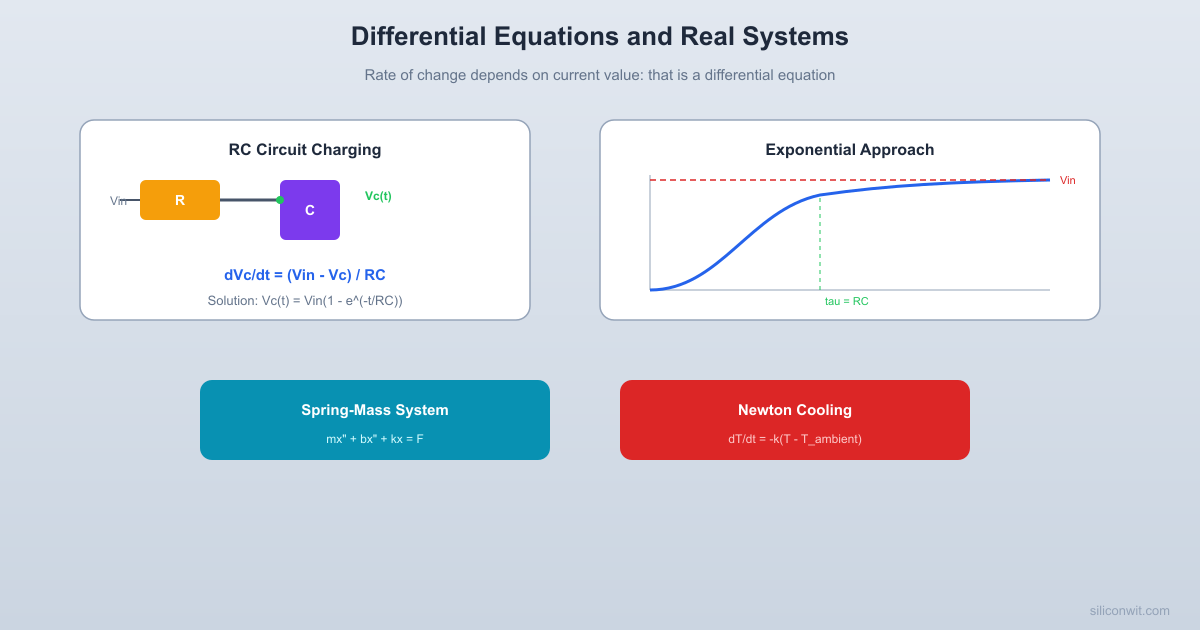
The RC Circuit: A First-Order System

The most important first-order ODE in electronics. A resistor in series with a capacitor , driven by a voltage source .

        R
  Vin --/\/\/\--+-- Vout
                 |
                 = C
                 |
  GND -----------+

Kirchhoff’s voltage law gives:

The current through the capacitor is . Substituting:

Rearranging:

This is the standard first-order ODE. The rate of change of is proportional to the difference between the input and the current value. The product is the time constant: the characteristic time scale of the system.

The Solution

If is a constant (step input) and the capacitor starts at :

After one time constant (), the capacitor has charged to about 63% of . After , it is within 1% of fully charged.

Why This Matters Everywhere

The RC equation is not just about capacitors. Any system where the rate of approach to equilibrium is proportional to the distance from equilibrium follows this same equation. A thermocouple responding to a temperature change. A sensor settling to a new value. A tank filling through a pipe. The math is identical; only the physical variables change.

Newton’s Law of Cooling: Your Coffee Cup

Newton observed that a hot object cools at a rate proportional to the temperature difference between the object and its surroundings:

This is the same structure as the RC circuit. The solution is the same shape:

The constant depends on the thermal properties: surface area, material, air circulation. A ceramic mug cools faster than a vacuum flask because is larger.

The interest on your savings account follows this same exponential equation, just growing instead of decaying. Compound interest is , the same mathematical structure as a charging capacitor. The constants differ, but the equation is identical.

import numpy as np
import matplotlib.pyplot as plt

# Compare cooling in different containers
T_ambient = 22  # room temperature (C)
T_0 = 90        # initial coffee temperature (C)
t = np.linspace(0, 120, 500)  # 2 hours

# Different cooling constants (1/min)
containers = {
    'Open cup': 0.04,
    'Ceramic mug': 0.025,
    'Travel mug': 0.008,
    'Vacuum flask': 0.002
}

plt.figure(figsize=(8, 5))
for name, k in containers.items():
    T = T_ambient + (T_0 - T_ambient) * np.exp(-k * t)
    plt.plot(t, T, linewidth=2, label=f'{name} (k={k})')

plt.axhline(y=60, color='gray', linestyle=':', alpha=0.5, label='Drinkable (~60 C)')
plt.xlabel('Time (minutes)')
plt.ylabel('Temperature (C)')
plt.title("Newton's Law of Cooling")
plt.legend()
plt.grid(True, alpha=0.3)
plt.tight_layout()
plt.show()

The Spring-Mass System: A Second-Order ODE

Attach a mass to a spring with stiffness . Pull it and release. Newton’s second law gives:

where is the damping coefficient (friction) and is an external force. The dots are shorthand: and .

  Wall
  |
  |/\/\/\/\/\---[  M  ]----->  x
  |   spring k    mass m
  |
  |~~~~~~~~~~~~~ damper b (friction)

Your car’s suspension is exactly this system. The spring supports the car’s weight, the shock absorber provides damping, and the car body is the mass. Too little damping (worn shocks) means a bouncy ride. Too much damping means a harsh ride that transmits every bump. The manufacturer tunes the suspension to be slightly underdamped for a comfortable balance of smoothness and responsiveness.

This is the second-order ODE that governs vibration in mechanical systems, oscillation in electrical circuits, and resonance in acoustic systems. The three terms represent:

• : inertia (mass resists acceleration)
• : damping (friction opposes velocity)
• : restoring force (spring pulls back toward equilibrium)

Natural Frequency and Damping Ratio

The two key parameters are:

The natural frequency tells you how fast the system wants to oscillate. The damping ratio tells you how quickly oscillations die out.

Python: Damping Regimes

import numpy as np
import matplotlib.pyplot as plt

# Spring-mass parameters
omega_n = 2 * np.pi  # natural frequency (rad/s), about 1 Hz
t = np.linspace(0, 5, 1000)

# Different damping ratios
damping_cases = {
    'Underdamped (zeta=0.1)': 0.1,
    'Underdamped (zeta=0.3)': 0.3,
    'Critically damped (zeta=1.0)': 1.0,
    'Overdamped (zeta=2.0)': 2.0,
}

plt.figure(figsize=(10, 6))
for label, zeta in damping_cases.items():
    if zeta < 1:
        omega_d = omega_n * np.sqrt(1 - zeta**2)
        x = np.exp(-zeta * omega_n * t) * np.cos(omega_d * t)
    elif zeta == 1:
        x = (1 + omega_n * t) * np.exp(-omega_n * t)
    else:
        r1 = -omega_n * (zeta + np.sqrt(zeta**2 - 1))
        r2 = -omega_n * (zeta - np.sqrt(zeta**2 - 1))
        # Initial conditions: x(0)=1, v(0)=0
        c2 = (r1) / (r1 - r2)
        c1 = 1 - c2
        x = c1 * np.exp(r1 * t) + c2 * np.exp(r2 * t)
    plt.plot(t, x, linewidth=2, label=label)

plt.axhline(y=0, color='k', linewidth=0.5)
plt.xlabel('Time (s)')
plt.ylabel('Displacement')
plt.title('Spring-Mass System: Damping Regimes')
plt.legend()
plt.grid(True, alpha=0.3)
plt.tight_layout()
plt.show()

Solving ODEs Numerically: Euler’s Method

Most differential equations have no closed-form solution. The RC circuit and spring-mass system are special because their solutions can be written as exponentials and sines. In practice, you solve ODEs numerically.

The simplest numerical method is Euler’s method. The idea is direct:

1. You know at time

2. The ODE tells you at that point

3. Step forward a small amount:

4. Repeat from the new point

That is it. You are walking along the solution curve by following the tangent line for a small step, then recalculating the slope.

Euler’s Method for the RC Circuit

import numpy as np
import matplotlib.pyplot as plt

# RC circuit parameters
R = 10e3     # 10 kohm
C = 100e-6   # 100 uF
tau = R * C  # time constant = 1 second
V_in = 5.0   # 5V step input

# Euler's method
dt = 0.01    # time step (seconds)
t_end = 5.0  # simulate 5 seconds
N = int(t_end / dt)

t = np.zeros(N)
V = np.zeros(N)
V[0] = 0  # capacitor starts discharged

for i in range(N - 1):
    dVdt = (V_in - V[i]) / tau
    V[i+1] = V[i] + dVdt * dt
    t[i+1] = t[i] + dt

# Exact solution for comparison
t_exact = np.linspace(0, t_end, 500)
V_exact = V_in * (1 - np.exp(-t_exact / tau))

plt.figure(figsize=(8, 5))
plt.plot(t_exact, V_exact, 'b-', linewidth=2, label='Exact solution')
plt.plot(t[::10], V[::10], 'ro', markersize=4, label=f'Euler (dt={dt}s)')
plt.xlabel('Time (s)')
plt.ylabel('Capacitor Voltage (V)')
plt.title('RC Circuit: Euler Method vs Exact Solution')
plt.legend()
plt.grid(True, alpha=0.3)
plt.tight_layout()
plt.show()

print(f"Time constant: {tau:.3f} s")
print(f"At t=tau: exact={V_in*(1-np.exp(-1)):.3f}V, "
      f"Euler={V[int(tau/dt)]:.3f}V")

Converting Second-Order to First-Order

Euler’s method handles first-order ODEs directly. To solve the spring-mass system (second-order), convert it into two first-order equations:

Let (velocity). Then:

Now you have two coupled first-order ODEs, which Euler’s method can handle by updating both and at each step.

Euler’s Method for the Spring-Mass System

import numpy as np
import matplotlib.pyplot as plt

# Spring-mass parameters
m = 1.0     # mass (kg)
k = 10.0    # spring constant (N/m)
b = 0.5     # damping coefficient (N*s/m)
F = 0.0     # no external force

omega_n = np.sqrt(k / m)
zeta = b / (2 * np.sqrt(k * m))
print(f"Natural frequency: {omega_n:.2f} rad/s ({omega_n/(2*np.pi):.2f} Hz)")
print(f"Damping ratio: {zeta:.3f}")

# Euler's method
dt = 0.005
t_end = 10.0
N = int(t_end / dt)

t = np.zeros(N)
x = np.zeros(N)
v = np.zeros(N)

# Initial conditions: pulled 1 meter and released
x[0] = 1.0
v[0] = 0.0

for i in range(N - 1):
    ax = (F - b * v[i] - k * x[i]) / m  # acceleration
    x[i+1] = x[i] + v[i] * dt
    v[i+1] = v[i] + ax * dt
    t[i+1] = t[i] + dt

plt.figure(figsize=(10, 5))
plt.plot(t, x, 'b-', linewidth=1.5)
plt.xlabel('Time (s)')
plt.ylabel('Position (m)')
plt.title(f'Spring-Mass System (zeta={zeta:.2f}, f_n={omega_n/(2*np.pi):.2f} Hz)')
plt.grid(True, alpha=0.3)
plt.tight_layout()
plt.show()

When Euler’s Method Fails

Euler’s method is simple but not always reliable. Two common problems:

Instability. If the time step is too large relative to the system’s time constant, the solution blows up. For the RC circuit, you need for stability. For stiff systems (systems with very fast and very slow dynamics), the required step size can be impractically small.

Drift. Euler’s method accumulates error over time. For the spring-mass system, it slowly adds energy: the oscillation amplitude grows instead of staying constant or decaying. Better methods like the Runge-Kutta method (covered in the Numerical Methods lesson) fix this.

import numpy as np
import matplotlib.pyplot as plt

# Show Euler instability with large time step
tau = 1.0
V_in = 5.0

fig, axes = plt.subplots(1, 3, figsize=(12, 4))
dt_values = [0.1, 0.5, 2.5]

for ax, dt in zip(axes, dt_values):
    N = int(5.0 / dt) + 1
    t = np.zeros(N)
    V = np.zeros(N)
    for i in range(N - 1):
        V[i+1] = V[i] + (V_in - V[i]) / tau * dt
        t[i+1] = t[i] + dt

    t_exact = np.linspace(0, 5, 200)
    V_exact = V_in * (1 - np.exp(-t_exact / tau))

    ax.plot(t_exact, V_exact, 'b-', linewidth=2, label='Exact')
    ax.plot(t, V, 'ro-', markersize=4, label=f'Euler')
    ax.set_title(f'dt = {dt}s (dt/tau = {dt/tau})')
    ax.set_xlabel('Time (s)')
    ax.set_ylim(-2, 10)
    ax.legend(fontsize=8)
    ax.grid(True, alpha=0.3)

axes[0].set_ylabel('Voltage (V)')
plt.suptitle('Euler Method: Effect of Time Step Size', fontsize=12)
plt.tight_layout()
plt.show()

From ODEs to System Modeling

Differential equations are the bridge between physical laws and predictions. The process:

1. Identify the physical laws governing the system (Newton’s law, Kirchhoff’s law, conservation of energy)

2. Write the governing equation as an ODE

3. Identify the parameters (, , , , )

4. Solve analytically if possible, numerically if not

5. Validate by comparing predictions to measured data

This is exactly the workflow used in the Modeling and Simulation course, where these techniques are applied to mechanical, electrical, and thermal systems in detail.

Exercises

1. RC time constant. An RC circuit has and . What is the time constant? If and the capacitor starts discharged, how long until reaches 3.0 V?

2. Cooling experiment. Measure the temperature of a cup of hot water every minute for 30 minutes. Fit Newton’s cooling law to your data to find . How well does the exponential model match?

3. Step size sensitivity. Solve the RC circuit with Euler’s method using , , , , and . Plot all solutions on the same graph. At what step size does the error become unacceptable? At what step size does the solution become unstable?

4. Damped oscillator. Use Euler’s method to simulate a spring-mass system with , , and three different damping values: , , . What is in each case? How do the time histories differ?

5. Coupled systems. Two RC circuits in series (the output of the first feeds the input of the second). Write the system of two coupled first-order ODEs and solve numerically. How does the response differ from a single RC circuit?

References

• Strogatz, S. H. (2015). Nonlinear Dynamics and Chaos. Westview Press. Chapter 2 is an excellent introduction to first-order ODEs.
• Zill, D. G. (2017). A First Course in Differential Equations with Modeling Applications. Cengage.
• 3Blue1Brown. Differential Equations. youtube.com/playlist?list=PLZHQObOWTQDNPOjrT6KVlfJuKtYTftqH6