Mechanical System Dynamics

Modified: Mar. 15, 2026

Published: Mar. 3, 2026

The spring-mass-damper system is the mechanical equivalent of the RLC circuit from the previous lesson. It appears everywhere: vehicle suspensions, vibration isolation mounts, mechanical shock absorbers, and even the compliance in robotic joints. In this lesson you will simulate it in Python, sweep the damping ratio to see all three regimes, build phase portraits, and create a suspension tuner that finds the optimal damping for your specific system. #MechanicalDynamics #Suspension #PythonSimulation

What We Are Building

Suspension Tuner

A Python tool that models a quarter-car suspension system. You specify the sprung mass, spring stiffness, and a range of damping coefficients. The tool simulates the response to a road bump, sweeps the damping ratio, and identifies the optimal value that minimizes settling time while keeping overshoot below a target threshold. It also generates phase portraits showing the system’s trajectory in state space.

Project specifications:

Parameter	Value
System	Single-DOF spring-mass-damper (quarter-car model)
Input	Step displacement (road bump)
Sweep Variable	Damping coefficient (and damping ratio )
Outputs	Displacement vs. time, phase portrait, settling time vs. damping ratio
Optimization	Find that minimizes 2% settling time

The Physics

Equation of Motion

       +-------+
       |   m   |  <-- sprung mass (car body)
       +---+---+
           |
         -----   spring (k)
         /\/\/
           |
         -----   damper (c)
         |   |
           |
  ////////////////////  <-- ground (road surface)

Newton’s second law applied to the mass:

where is the displacement from equilibrium, is the mass, is the damping coefficient, and is the spring stiffness.

For a deeper look at the differential equations governing systems like this, see Applied Mathematics: Differential Equations in Real Systems.

To use solve_ivp, we convert this second-order ODE into two first-order ODEs by introducing the velocity :

Key Parameters

The natural frequency (undamped):

The damping ratio:

The critical damping coefficient:

Damping Ratio	Behavior	Physical Example
	Undamped, oscillates forever	Ideal spring (no friction)
	Underdamped, oscillates and decays	Typical car suspension
	Critically damped, fastest non-oscillatory	Door closer mechanism
	Overdamped, returns slowly without oscillation	Heavy hydraulic damper

Energy in the System

At any instant, the system has kinetic energy and potential energy:

For an undamped system (), total energy is conserved. For a damped system, energy is dissipated by the damper at a rate .

Complete Python Code

Save this as suspension_tuner.py:

"""
Suspension Tuner
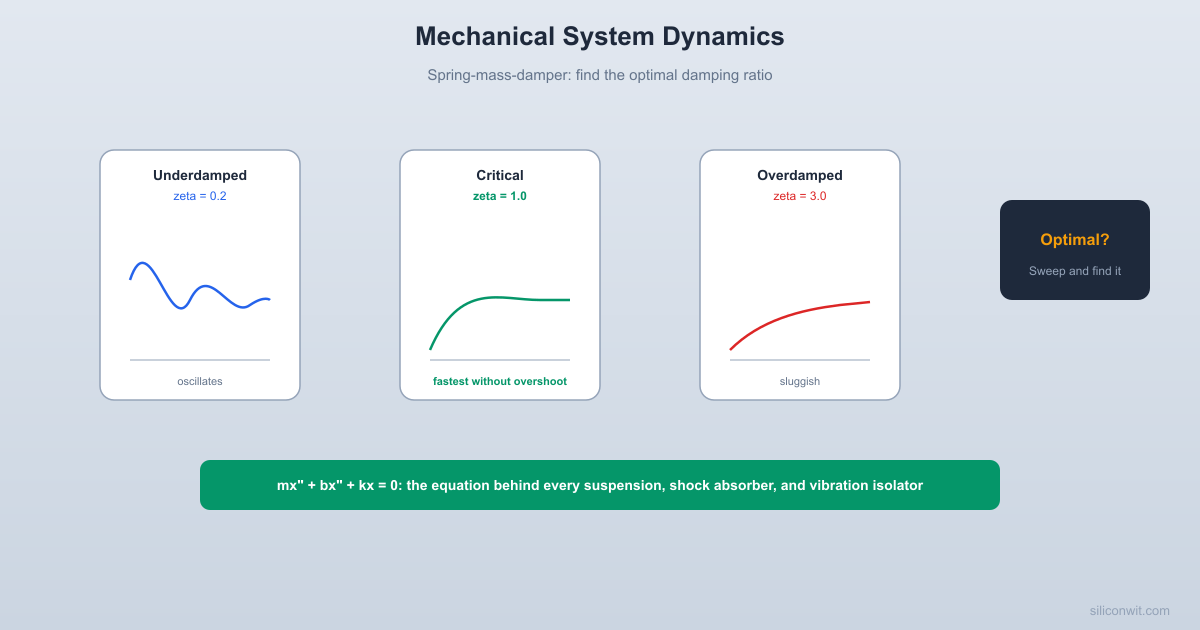
Models a spring-mass-damper system, sweeps damping ratio,
and finds the optimal damping for minimum settling time.
"""

import numpy as np
from scipy.integrate import solve_ivp
import matplotlib.pyplot as plt

# -------------------------------------------------------
# System parameters (quarter-car model)
# -------------------------------------------------------
MASS = 250.0        # Sprung mass in kg (quarter of a 1000 kg car)
STIFFNESS = 15000.0 # Spring stiffness in N/m
X0 = 0.05           # Initial displacement in meters (5 cm bump)
V0 = 0.0            # Initial velocity in m/s

# Derived parameters
OMEGA_N = np.sqrt(STIFFNESS / MASS)
C_CRITICAL = 2 * np.sqrt(STIFFNESS * MASS)
F_N = OMEGA_N / (2 * np.pi)

print("=" * 55)
print("  SUSPENSION SYSTEM PARAMETERS")
print("=" * 55)
print(f"  Mass:                {MASS:.0f} kg")
print(f"  Spring stiffness:    {STIFFNESS:.0f} N/m")
print(f"  Natural frequency:   {F_N:.2f} Hz ({OMEGA_N:.2f} rad/s)")
print(f"  Critical damping:    {C_CRITICAL:.0f} N*s/m")
print(f"  Initial bump:        {X0*100:.1f} cm")
print("=" * 55)

def spring_mass_damper_ode(t, y, c):
    """
    ODE for spring-mass-damper system.
    y = [x, v] where x is displacement and v is velocity.
    """
    x, v = y
    dxdt = v
    dvdt = -(c / MASS) * v - (STIFFNESS / MASS) * x
    return [dxdt, dvdt]

def simulate(c, t_end=2.0, n_points=2000):
    """
    Simulate the system with damping coefficient c.
    Returns time, displacement, velocity arrays.
    """
    sol = solve_ivp(
        lambda t, y: spring_mass_damper_ode(t, y, c),
        [0, t_end],
        [X0, V0],
        dense_output=True,
        max_step=t_end / 1000
    )
    t = np.linspace(0, t_end, n_points)
    y = sol.sol(t)
    return t, y[0], y[1]

def find_settling_time(t, x, threshold_fraction=0.02):
    """
    Find the 2% settling time: the last time the displacement
    exceeds 2% of the initial displacement.
    """
    threshold = threshold_fraction * abs(X0)
    settled = np.abs(x) < threshold

    if not np.any(settled):
        return t[-1]  # Never settled within simulation window

    # Find the last time it was NOT settled
    not_settled = np.where(~settled)[0]
    if len(not_settled) == 0:
        return 0.0
    last_unsettled_idx = not_settled[-1]

    if last_unsettled_idx >= len(t) - 1:
        return t[-1]

    return t[last_unsettled_idx + 1]

def find_overshoot(x):
    """
    Find the percent overshoot (maximum excursion beyond zero
    on the opposite side of the initial displacement).
    """
    # For a system starting at positive X0 and settling to 0,
    # overshoot is the maximum negative excursion
    min_x = np.min(x)
    if min_x < 0:
        return abs(min_x) / X0 * 100.0
    return 0.0

# -------------------------------------------------------
# 1. Compare three damping regimes
# -------------------------------------------------------
def plot_three_regimes():
    """Plot underdamped, critically damped, and overdamped responses."""

    zeta_values = [0.2, 0.5, 1.0, 2.0]
    colors = ["tab:red", "tab:blue", "tab:green", "tab:purple"]
    labels = [
        "zeta=0.2 (underdamped)",
        "zeta=0.5 (underdamped)",
        "zeta=1.0 (critically damped)",
        "zeta=2.0 (overdamped)"
    ]

    fig, axes = plt.subplots(1, 2, figsize=(14, 5))
    fig.suptitle("Spring-Mass-Damper: Effect of Damping Ratio",
                 fontsize=13, fontweight="bold")

    for zeta, color, label in zip(zeta_values, colors, labels):
        c = zeta * C_CRITICAL
        t, x, v = simulate(c, t_end=2.0)

        # Time response
        axes[0].plot(t, x * 100, color=color, linewidth=2, label=label)

        # Phase portrait
        axes[1].plot(x * 100, v * 100, color=color, linewidth=1.5, label=label)
        axes[1].plot(x[0] * 100, v[0] * 100, "o", color=color, markersize=6)

    # Time response formatting
    axes[0].axhline(y=0, color="black", linewidth=0.5)
    axes[0].set_xlabel("Time (s)")
    axes[0].set_ylabel("Displacement (cm)")
    axes[0].set_title("Step Response")
    axes[0].legend(fontsize=8)
    axes[0].grid(True, alpha=0.3)

    # Phase portrait formatting
    axes[1].plot(0, 0, "kx", markersize=10, markeredgewidth=2)  # Equilibrium
    axes[1].set_xlabel("Displacement (cm)")
    axes[1].set_ylabel("Velocity (cm/s)")
    axes[1].set_title("Phase Portrait")
    axes[1].legend(fontsize=8)
    axes[1].grid(True, alpha=0.3)

    plt.tight_layout()
    plt.savefig("damping_comparison.png", dpi=150, bbox_inches="tight")
    plt.show()
    print("Saved: damping_comparison.png\n")

# -------------------------------------------------------
# 2. Energy dissipation over time
# -------------------------------------------------------
def plot_energy():
    """Show how energy is dissipated for different damping ratios."""

    zeta_values = [0.1, 0.5, 1.0]
    colors = ["tab:red", "tab:blue", "tab:green"]

    fig, axes = plt.subplots(1, 3, figsize=(14, 4))
    fig.suptitle("Energy Dissipation in Spring-Mass-Damper System",
                 fontsize=13, fontweight="bold")

    for idx, (zeta, color) in enumerate(zip(zeta_values, colors)):
        c = zeta * C_CRITICAL
        t, x, v = simulate(c, t_end=3.0)

        ke = 0.5 * MASS * v**2
        pe = 0.5 * STIFFNESS * x**2
        total = ke + pe

        axes[idx].fill_between(t, 0, ke, alpha=0.4, color="tab:orange",
                                label="Kinetic")
        axes[idx].fill_between(t, ke, ke + pe, alpha=0.4, color="tab:cyan",
                                label="Potential")
        axes[idx].plot(t, total, "k--", linewidth=1, label="Total",
                        alpha=0.7)
        axes[idx].set_xlabel("Time (s)")
        axes[idx].set_ylabel("Energy (J)")
        axes[idx].set_title(f"zeta = {zeta}")
        axes[idx].legend(fontsize=7)
        axes[idx].grid(True, alpha=0.3)
        axes[idx].set_ylim(bottom=0)

    plt.tight_layout()
    plt.savefig("energy_dissipation.png", dpi=150, bbox_inches="tight")
    plt.show()
    print("Saved: energy_dissipation.png\n")

# -------------------------------------------------------
# 3. Sweep damping ratio and find optimal
# -------------------------------------------------------
def sweep_and_optimize():
    """
    Sweep zeta from 0.1 to 3.0, compute settling time and overshoot
    for each value, and find the optimal damping ratio.
    """

    zeta_range = np.linspace(0.1, 3.0, 200)
    settling_times = []
    overshoots = []

    for zeta in zeta_range:
        c = zeta * C_CRITICAL
        t, x, v = simulate(c, t_end=5.0, n_points=5000)
        ts = find_settling_time(t, x, threshold_fraction=0.02)
        os_pct = find_overshoot(x)
        settling_times.append(ts)
        overshoots.append(os_pct)

    settling_times = np.array(settling_times)
    overshoots = np.array(overshoots)

    # Find optimal: minimum settling time
    idx_opt = np.argmin(settling_times)
    zeta_opt = zeta_range[idx_opt]
    ts_opt = settling_times[idx_opt]
    os_opt = overshoots[idx_opt]

    print("=" * 55)
    print("  OPTIMIZATION RESULTS")
    print("=" * 55)
    print(f"  Optimal damping ratio:  {zeta_opt:.3f}")
    print(f"  Optimal damping coeff:  {zeta_opt * C_CRITICAL:.0f} N*s/m")
    print(f"  Settling time (2%):     {ts_opt*1000:.0f} ms")
    print(f"  Overshoot:              {os_opt:.1f}%")
    print("=" * 55)

    # Also find optimal with overshoot constraint (< 10%)
    mask = overshoots < 10.0
    if np.any(mask):
        constrained_settling = settling_times.copy()
        constrained_settling[~mask] = np.inf
        idx_constrained = np.argmin(constrained_settling)
        zeta_constrained = zeta_range[idx_constrained]
        ts_constrained = settling_times[idx_constrained]
        os_constrained = overshoots[idx_constrained]
        print(f"\n  With overshoot < 10% constraint:")
        print(f"  Optimal damping ratio:  {zeta_constrained:.3f}")
        print(f"  Settling time (2%):     {ts_constrained*1000:.0f} ms")
        print(f"  Overshoot:              {os_constrained:.1f}%")
        print("=" * 55)

    # Plot
    fig, axes = plt.subplots(1, 2, figsize=(12, 5))
    fig.suptitle("Suspension Tuning: Damping Ratio Sweep",
                 fontsize=13, fontweight="bold")

    # Settling time vs zeta
    axes[0].plot(zeta_range, settling_times * 1000, "tab:blue", linewidth=2)
    axes[0].axvline(x=zeta_opt, color="red", linestyle="--", alpha=0.7,
                     label=f"Optimal: zeta={zeta_opt:.3f}")
    axes[0].axvline(x=1.0, color="gray", linestyle=":", alpha=0.5,
                     label="Critical damping")
    axes[0].set_xlabel("Damping Ratio (zeta)")
    axes[0].set_ylabel("2% Settling Time (ms)")
    axes[0].set_title("Settling Time vs. Damping Ratio")
    axes[0].legend(fontsize=8)
    axes[0].grid(True, alpha=0.3)

    # Overshoot vs zeta
    axes[1].plot(zeta_range, overshoots, "tab:orange", linewidth=2)
    axes[1].axhline(y=10, color="red", linestyle="--", alpha=0.5,
                     label="10% overshoot limit")
    axes[1].axvline(x=1.0, color="gray", linestyle=":", alpha=0.5,
                     label="Critical damping")
    axes[1].set_xlabel("Damping Ratio (zeta)")
    axes[1].set_ylabel("Overshoot (%)")
    axes[1].set_title("Overshoot vs. Damping Ratio")
    axes[1].legend(fontsize=8)
    axes[1].grid(True, alpha=0.3)

    plt.tight_layout()
    plt.savefig("suspension_tuning.png", dpi=150, bbox_inches="tight")
    plt.show()
    print("Saved: suspension_tuning.png\n")

    # Plot the optimal response
    c_opt = zeta_opt * C_CRITICAL
    t, x, v = simulate(c_opt, t_end=2.0)

    fig, ax = plt.subplots(figsize=(10, 4))
    ax.plot(t, x * 100, "tab:blue", linewidth=2,
            label=f"Optimal (zeta={zeta_opt:.3f})")

    # Compare with critical and a typical underdamped
    for zeta, color, label in [(0.3, "tab:red", "zeta=0.3"),
                                (1.0, "tab:green", "zeta=1.0")]:
        c = zeta * C_CRITICAL
        t2, x2, _ = simulate(c, t_end=2.0)
        ax.plot(t2, x2 * 100, color=color, linewidth=1.5,
                linestyle="--", label=label, alpha=0.7)

    ax.axhline(y=0, color="black", linewidth=0.5)
    ax.axhline(y=X0 * 100 * 0.02, color="gray", linestyle=":",
               alpha=0.4, label="2% band")
    ax.axhline(y=-X0 * 100 * 0.02, color="gray", linestyle=":",
               alpha=0.4)
    ax.set_xlabel("Time (s)")
    ax.set_ylabel("Displacement (cm)")
    ax.set_title("Optimal Suspension Response vs. Alternatives",
                 fontweight="bold")
    ax.legend(fontsize=8)
    ax.grid(True, alpha=0.3)

    plt.tight_layout()
    plt.savefig("optimal_response.png", dpi=150, bbox_inches="tight")
    plt.show()
    print("Saved: optimal_response.png")

# -------------------------------------------------------
# Main
# -------------------------------------------------------
if __name__ == "__main__":
    plot_three_regimes()
    plot_energy()
    sweep_and_optimize()

Running the Suspension Tuner

python suspension_tuner.py

The script produces three sets of plots:

Damping comparison showing underdamped, critically damped, and overdamped responses side by side, with phase portraits
Energy dissipation showing how kinetic and potential energy trade off and decay over time
Suspension tuning showing settling time and overshoot as functions of damping ratio, plus the optimal response

Reading the Phase Portrait

A phase portrait plots velocity against displacement. It reveals the system’s dynamics in a way that a time-domain plot cannot.

The trajectory spirals inward toward the equilibrium point at the origin. Each loop represents one oscillation cycle, and the spiral tightens as energy is dissipated. Lower damping means more loops.

  velocity
    ^
    |    .  .
    |   .    .
    |  .      .
    | .   (0,0) .  <-- equilibrium
    |  .      .
    |   .    .
    |    .  .
    +--------------> displacement

Why the Optimal Damping Is Not Exactly 1.0

A common misconception is that critical damping () gives the fastest settling. In practice, the optimal damping ratio depends on how you define “settled.”

For the 2% settling time criterion, the optimal value is typically around to . At this damping level, there is a small overshoot (less than 5%), but the system enters the 2% band faster than the critically damped case because the slight oscillation helps “push” the displacement toward zero.

This is exactly the same tradeoff that appears in PID control tuning (Lesson 5). Allowing a small overshoot often gives you a faster response.

Experiments to Try

Change the Mass

Double the mass to 500 kg. The natural frequency drops and the system responds more slowly. Notice that the optimal does not change much; it is a dimensionless ratio that captures the dynamics regardless of scale.

Forced Vibration

Add a sinusoidal forcing function: . Sweep near and observe resonance. The amplitude at resonance depends on .

Nonlinear Spring

Replace the linear spring with a hardening spring: . The response is no longer symmetric, and the resonance frequency shifts with amplitude.

Road Profile Input

Instead of a step input, use a realistic road profile (e.g., a sine wave plus noise). Evaluate ride comfort using the RMS acceleration of the sprung mass.

Key Takeaways

The spring-mass-damper is the same math as the RLC circuit

Replace , , , and you get the same second-order ODE. This analogy means everything you learn about mechanical damping applies to electrical circuits and vice versa.
Phase portraits reveal dynamics that time plots hide

The spiral shape tells you about energy dissipation, oscillation frequency, and stability at a glance.
Optimal damping depends on your performance criteria

If you care about overshoot, choose . If you care about settling time, the optimum is near . There is always a tradeoff.
Sweeping parameters is cheap in simulation

Testing 200 damping values took less than a second. On real hardware, each test would require swapping a physical damper. This is why you simulate first.

Next Lesson

In the next lesson, we move from mechanical to thermal systems. You will build thermal resistance networks for electronic components and create a heatsink sizer that tells you whether your chip stays within its safe operating temperature.

Thermal Modeling for Electronics →

Comments

Loading comments...