Trajectory planning bridges the gap between knowing where a robot should go and actually getting it there smoothly. In this lesson, we design trajectories for a warehouse mobile manipulator performing pick-and-place operations, covering polynomial interpolation, spline paths through multiple waypoints, and trapezoidal velocity profiles that respect actuator limits. #TrajectoryPlanning #MotionControl #Robotics
Learning Objectives
By the end of this lesson, you will be able to:
Compare joint-space and task-space trajectory planning approaches and select the appropriate one for a given task
Derive cubic and quintic polynomial trajectories with specified boundary conditions
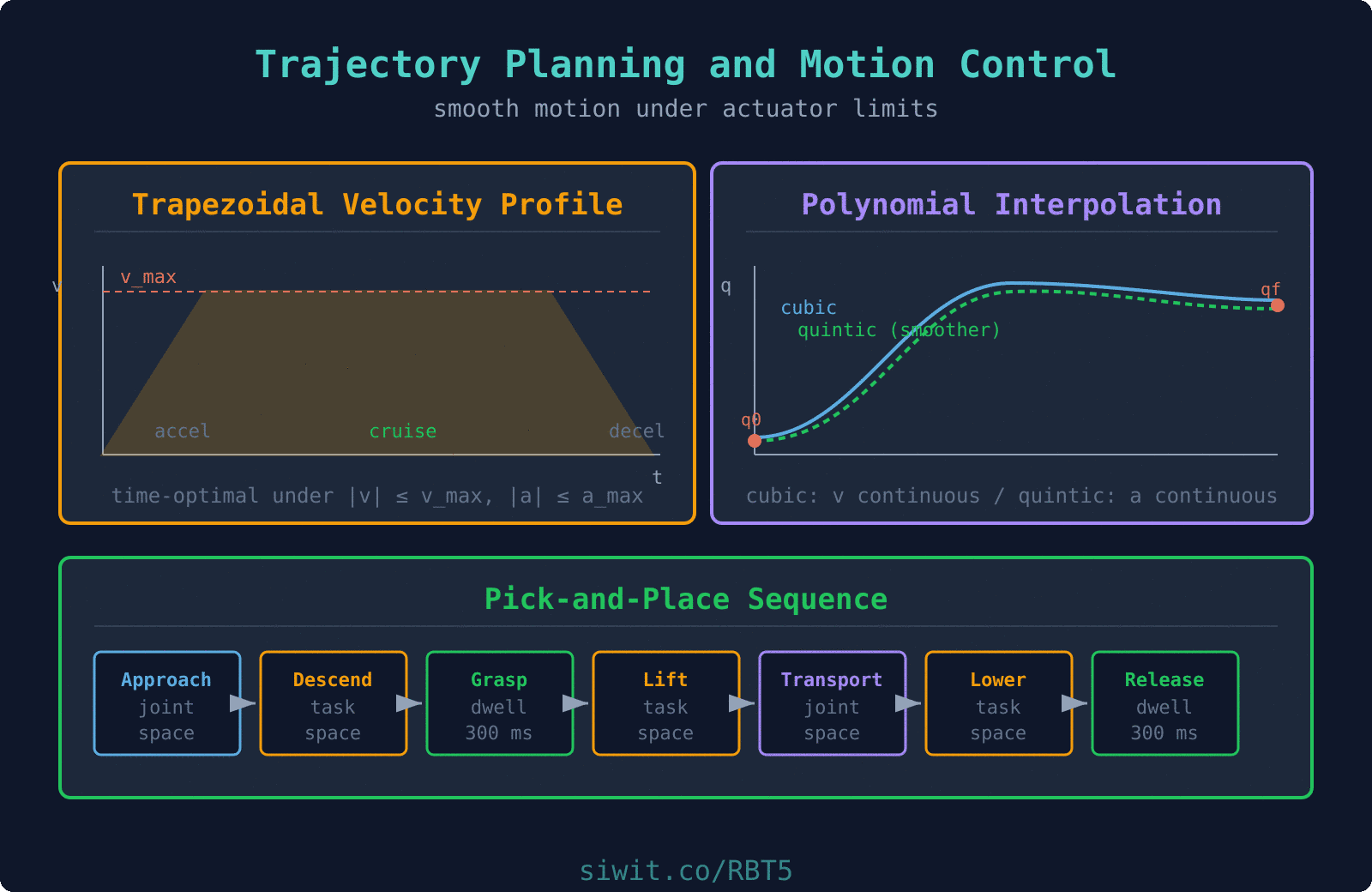
Implement trapezoidal velocity profiles that respect actuator velocity and acceleration limits
Construct spline trajectories through multiple via points with continuous velocity and acceleration
Sequence a complete pick-and-place operation with approach, grasp, transport, place, and return phases
Real-World Engineering Challenge: Warehouse Mobile Manipulator Pick-and-Place
A warehouse mobile manipulator must pick boxes from storage shelves and place them on a conveyor belt for shipping. The robot arm (a 6-DOF articulated manipulator mounted on a mobile base) needs to move between shelf locations and the conveyor with smooth, predictable motions. Jerky trajectories cause the gripper to drop boxes, damage products, and wear out actuators prematurely. The system must handle boxes at different shelf heights, plan paths that avoid shelf edges, and maintain a cycle time under 8 seconds per pick-and-place operation.
Why Trajectory Smoothness Matters
A trajectory that commands instantaneous velocity changes requires infinite acceleration, which no real motor can produce. The result is vibration, tracking error, and mechanical stress. Smooth trajectories (with continuous velocity, and ideally continuous acceleration) let the motor controllers track the commanded path accurately, reduce energy consumption, and extend the lifespan of gears and bearings. In a warehouse setting, a single dropped box can halt an entire packing line, so smoothness directly affects throughput and reliability.
Fundamental Theory
Joint-Space vs. Task-Space Trajectory Planning
There are two fundamental approaches to planning a robot trajectory. Joint-space planning interpolates directly between joint angle vectors, while task-space planning interpolates the end-effector pose (position and orientation) in Cartesian coordinates. Each approach has distinct advantages and trade-offs.
How it works: Given start joint angles and goal joint angles , interpolate each joint independently as a function of time .
Advantages:
Simple to implement: each joint follows its own polynomial or profile
No singularity issues during motion (the Jacobian is never needed)
Guaranteed to respect joint limits if start and goal are within limits
Computationally inexpensive
Disadvantages:
The end-effector path in Cartesian space is generally curved and unpredictable
Cannot guarantee straight-line motion of the tool tip
Not suitable when the Cartesian path matters (e.g., welding a seam, avoiding obstacles)
Best for: Point-to-point moves where only the start and end positions matter, such as moving between widely separated waypoints in a pick-and-place cycle.
How it works: Given start pose and goal pose in Cartesian space, interpolate position (and orientation using quaternion SLERP, covered in Orientation and Quaternions), then solve inverse kinematics at each time step.
Advantages:
Full control over the Cartesian path (straight lines, arcs, or any desired shape)
Essential for tasks where the path matters (painting, welding, deburring)
Easier to specify obstacle avoidance constraints
Disadvantages:
Requires solving inverse kinematics at every time step (computationally expensive)
May encounter singularities during the motion
Joint velocities can become very large near singular configurations
No guarantee that joint limits are respected along the path
Best for: Motions where the Cartesian path is critical, such as descending vertically onto a box or following a shelf edge.
Linear Interpolation: The Simplest Trajectory
The simplest trajectory linearly interpolates between start and goal:
The velocity is constant:
The problem: velocity jumps from zero to a constant value at and back to zero at . These discontinuities require infinite acceleration, which is physically impossible. Linear interpolation is useful only as a building block inside more sophisticated methods (like trapezoidal profiles).
Cubic Polynomial Interpolation
A cubic polynomial provides the minimum-degree trajectory that can satisfy four boundary conditions: position and velocity at both the start and end of the motion. This gives us smooth velocity transitions with zero velocity at the endpoints, which is exactly what we need for a robot that starts and stops at rest.
The cubic polynomial trajectory is:
with velocity and acceleration:
Boundary Conditions
For a rest-to-rest motion from to over time :
Coefficient Derivation
Applying the boundary conditions:
From :
From :
From and , solving the system:
Full derivation of the coefficient system
Starting from the four equations:
Substituting and into the last two equations:
From the velocity equation:
Substituting into the position equation:
And therefore:
Quintic Polynomial: Acceleration Continuity
A quintic (5th-degree) polynomial provides six boundary conditions: position, velocity, and acceleration at both endpoints. This ensures the acceleration profile is also smooth at the start and end of the motion, which reduces jerk (the derivative of acceleration) and produces even gentler motion.
For rest-to-rest motion with zero acceleration at endpoints (, , , ):
Trapezoidal Velocity Profile
  Trapezoidal Velocity Profile
  velocity    ^    |         +-----------------+  v_max ......|                 |..............    |        /|                 |\    |       / |                 | \    |      /  |                 |  \    |     /   |                 |   \    |    /    |                 |    \    |   /     |                 |     \    +--/------+-----------------+------\----> time    0  t_a                    t_a+t_c  t_f
       Phase 1    Phase 2       Phase 3       Accel      Cruise        Decel       (a_max)    (v = v_max)   (-a_max)
  If distance is too short to reach v_max,  the cruise phase vanishes and the profile  becomes triangular (accel then decel).
In industrial applications, actuators have hard limits on maximum velocity and maximum acceleration. The trapezoidal velocity profile is the time-optimal trajectory under these constraints. It consists of three phases: constant acceleration, constant velocity (cruise), and constant deceleration. The velocity profile looks like a trapezoid when plotted against time.
Given maximum velocity and maximum acceleration , the motion from to (with ) has:
Phase 1: Acceleration ()
Phase 2: Cruise ()
Phase 3: Deceleration ()
The timing parameters:
S-Curve Profiles: Adding a Jerk Limit
A trapezoidal profile has discontinuous acceleration at four places (start of accel, start of cruise, start of decel, end of decel). Each jump is an instantaneous step in acceleration, which means infinite jerk (). For delicate payloads (electronics, surgical tools, full cups of liquid) this is unacceptable: the sudden acceleration change feels like a hammer blow at the attachment.
The fix is the S-curve (or seven-segment) profile, which adds constant-jerk ramps to each corner of the trapezoid. The velocity curve has a characteristic S shape at each end. You specify a third limit alongside and , and the profile smoothly ramps acceleration up to , cruises at constant , ramps back to zero, cruises at , and mirrors the pattern for deceleration. Most industrial motion controllers (Siemens SIMATIC, Rockwell Kinetix, Beckhoff TwinCAT) ship with S-curve profile generators; implement one yourself only if you need custom behavior.
Beyond Trapezoidal: TOPP for Time-Optimal Paths
The trapezoidal profile is time-optimal for one joint at a time. For a full robot following a Cartesian path, the binding constraint at each point along the path is usually a different joint (or a different axis of the task frame), and the joint velocity / acceleration / torque limits are themselves configuration-dependent. Computing a true time-optimal profile under all these constraints simultaneously is a classical problem solved by Time-Optimal Path Parameterization (TOPP).
The current industrial standard is TOPP-RA (Pham & Pham, 2017): it discretizes the geometric path and solves a sequence of small linear programs to find the fastest possible time parameterization under joint-velocity, joint-acceleration, and optionally joint-torque bounds. You will find it in toppra (Python), Drake, and as the contopp option in MATLAB’s Robotics System Toolbox. If the question “how do I make this trajectory 10 percent faster without exceeding limits?” comes up, this is the tool.
Spline Interpolation Through Multiple Waypoints
When a trajectory must pass through multiple via points (for example, a sequence of shelf locations), we connect consecutive pairs with cubic polynomials and enforce continuity of position, velocity, and acceleration at each via point. This produces a cubic spline trajectory.
For waypoints at times , we construct cubic segments. At each interior waypoint , we require:
Position continuity: The segment ending at and the segment starting at agree on the position value.
Velocity continuity: (velocity from the left equals velocity from the right).
Acceleration continuity: (acceleration matches across the boundary).
With boundary conditions and (natural spline with rest at endpoints), this forms a tridiagonal linear system that can be solved efficiently.
Via-point velocity estimation
When time-stamps are given but intermediate velocities are not specified, a common heuristic is to set the velocity at each interior via point to the average of the linear velocities on either side:
If the two adjacent segments have opposite signs (the joint reverses direction), the via-point velocity is set to zero.
Pick-and-Place Task Phases
A complete pick-and-place operation is a sequence of trajectory segments, each designed for a specific purpose. The segments are connected end-to-end with matching positions and velocities at the transition points. Here is the full phase breakdown for our warehouse manipulator.
Move to approach position
Joint-space cubic polynomial from the home configuration to a position above the target box. This is a large free-space motion where the Cartesian path does not matter.
Descend to object
Task-space straight-line descent (vertical) from the approach position to the grasp position. This uses Cartesian trajectory planning with IK at each step to ensure the gripper approaches the box from directly above.
Grasp
Close the gripper. The arm holds position while the gripper actuates. Typical dwell time: 200-500 ms.
Lift
Task-space straight-line vertical lift to a safe clearance height above the shelf. This prevents the box from clipping the shelf edge.
Transport
Joint-space trajectory from the lifted position above the shelf to a position above the conveyor. This is the longest segment and should use a trapezoidal velocity profile for time-optimal motion.
Lower to placement
Task-space straight-line descent to the conveyor placement position.
Release
Open the gripper. Dwell time: 200-500 ms.
Return home
Joint-space trajectory back to the home configuration, ready for the next cycle.
Via Points and Blending
In practice, stopping at every via point (zero velocity) wastes time. Via-point blending replaces the stop-and-go transitions with smooth curves that pass near (but not exactly through) the via points. The robot trades a small amount of path accuracy for significant cycle time improvement.
A common blending approach defines a blend radius around each via point. Within the blend region, a parabolic (or circular) curve replaces the linear segment. Outside the blend regions, the robot follows the original straight-line segments at cruise velocity. The blend radius is chosen as a trade-off between path accuracy and transition smoothness.
Cartesian Straight-Line Motion
For task-space segments (descent, lift, placement), we generate a straight line in Cartesian space and convert to joint trajectories using the Jacobian, introduced in Velocity Kinematics and the Jacobian.
Given a desired Cartesian velocity , the required joint velocities are:
Or using the pseudoinverse for redundant robots:
The trajectory is generated by discretizing the Cartesian path into small steps and solving IK (or using the resolved-rate method above) at each step.
What If the Cartesian Path Is Infeasible?
A straight line in Cartesian space can demand joint velocities above actuator limits, especially near the workspace boundary or near a singularity where small Cartesian motion requires large joint motion. Before executing a task-space trajectory, validate it by sweeping along the path at your planned speed, computing at each step, and checking that every joint stays within [-v_max, v_max] and every acceleration stays within [-a_max, a_max].
If any step violates limits, you have three practical options:
Slow the trajectory globally: reduce the Cartesian cruise velocity until the worst joint is within limits. Easy to implement, costs time.
Reparameterize using TOPP: find the time-optimal speed profile along the fixed geometric path. Best if the path shape must be preserved.
Replan the path: move the via points away from the singular region, sacrificing a straight line for a curved but feasible motion. Best when the Cartesian shape is flexible.
Silently commanding unreachable velocities will either produce a tracking error (the robot falls behind) or trip the controller’s safety limits and halt the motion mid-task.
We now apply the trajectory planning tools to our warehouse mobile manipulator. The robot must pick a box from a shelf at height 1.2 m and place it on a conveyor at height 0.8 m. The arm has actuator limits of 120 deg/s maximum joint velocity and 300 deg/s² maximum joint acceleration. The target cycle time is under 8 seconds.
Trajectory strategy for each phase:
Phase
Planning Space
Method
Rationale
Move to approach
Joint space
Trapezoidal
Time-optimal, large motion
Descend to object
Task space
Cubic polynomial
Smooth vertical descent, short distance
Grasp (dwell)
None
Hold position
Gripper closes
Lift
Task space
Cubic polynomial
Smooth vertical lift
Transport
Joint space
Trapezoidal
Time-optimal, longest segment
Lower to placement
Task space
Cubic polynomial
Smooth vertical descent
Release (dwell)
None
Hold position
Gripper opens
Return home
Joint space
Trapezoidal
Time-optimal return
Cycle time budget:
Phase
Duration
Move to approach
1.2 s
Descend
0.5 s
Grasp dwell
0.3 s
Lift
0.5 s
Transport
2.5 s
Lower
0.5 s
Release dwell
0.3 s
Return home
1.5 s
Total
7.3 s
This is within the 8-second target. The transport phase dominates the cycle time, so optimizing this segment (higher cruise velocity, shorter acceleration time) has the greatest impact on throughput.
Improving cycle time further
Several strategies can reduce cycle time below 7 seconds:
Overlap phases: Begin closing the gripper while the arm is still completing the final descent. This saves 100-200 ms.
Via-point blending: Instead of coming to a full stop at the approach position, blend through it at reduced speed. The arm follows a smooth curve that passes close to the approach point without stopping.
Increase actuator limits: Higher-torque motors allow larger , which shortens the acceleration and deceleration phases of trapezoidal profiles.
Optimize waypoint placement: Position the approach and lift waypoints closer to the grasp point to minimize the descent and lift distances.
Design Guidelines
Match Method to Phase
Use trapezoidal velocity profiles for long free-space motions where time matters. Use polynomial interpolation for short, precise segments where smoothness is critical. Use task-space planning only when the Cartesian path is important (approach, descent, straight-line segments).
Always Check Actuator Limits
After generating any trajectory, compute the required joint velocities and accelerations and verify they are within the actuator ratings. For polynomial trajectories, the peak velocity and acceleration depend on the motion distance and duration. Shorter durations produce higher peaks.
Prefer Quintic for Delicate Payloads
When carrying fragile items (electronics, glass, food products), use quintic polynomials to ensure zero jerk at segment transitions. The additional computational cost is negligible compared to the cost of dropped or damaged goods.
Test Blending Radii in Simulation
Via-point blending trades path accuracy for speed. Always simulate the blended path and verify the maximum deviation from the nominal via points. For our warehouse application, a maximum deviation of 20 mm at via points is typically acceptable; for precision assembly, it may need to be under 0.1 mm.
Summary
Trajectory Planning Fundamentals
Joint-space planning is simple and singularity-free, while task-space planning provides Cartesian path control. Industrial systems combine both: joint-space for free motions, task-space for critical approach and departure segments.
Polynomial Interpolation
Cubic polynomials satisfy four boundary conditions (position and velocity at endpoints) and are the standard for smooth point-to-point motions. Quintic polynomials add acceleration continuity for even smoother transitions.
Trapezoidal Profiles
The trapezoidal velocity profile is time-optimal under velocity and acceleration constraints. It handles both the normal trapezoidal case (cruise phase present) and the degenerate triangular case (short distances).
Pick-and-Place Sequencing
A complete pick-and-place cycle is a sequence of trajectory segments, each chosen for its specific purpose. Proper phase sequencing, dwell times, and via-point blending determine the achievable cycle time and reliability.
Next lesson: We build complete Python robot simulations with 3D visualization, then connect the kinematic and trajectory planning tools from this course to real-world applications in manufacturing, logistics, medical robotics, and agricultural automation.
Comments