Simulating Electrical Circuits

Modified: Mar. 15, 2026

Published: Mar. 2, 2026

Every embedded system sits inside an electrical circuit, and understanding how circuits behave in the time and frequency domains is essential for hardware design. In this lesson you will simulate RC and RLC circuits in Python, verify that the simulation matches the analytical formulas you learned in school, and build a circuit analyzer that generates step responses and Bode plots from component values. #CircuitSimulation #BodePlot #Python

What We Are Building

RC/RLC Circuit Analyzer

A Python tool that accepts resistor, inductor, and capacitor values as inputs, then produces step response plots (voltage vs. time) and Bode plots (magnitude and phase vs. frequency). You can use it to predict how a filter or snubber will behave before you solder a single component.

Project specifications:

Parameter	Value
Circuit Types	Series RC, Series RLC
Step Response	Voltage across capacitor after a voltage step
Frequency Response	Bode plot (magnitude in dB, phase in degrees)
Solver	SciPy `solve_ivp` for time domain, analytical transfer function for frequency domain
Output	Step response plot, Bode plot, key parameters printed to console

RC Circuit Fundamentals

The Circuit

         R
  Vin ---/\/\/--- + ---
                  |    |
                  C    Vout
                  |    |
  GND ---------- + ---

When a voltage step is applied to an RC circuit, the capacitor charges exponentially. The governing equation comes from Kirchhoff’s voltage law:

Since , we get:

The time constant is . After one time constant, the capacitor reaches about 63.2% of the step voltage. After five time constants, it is effectively at the final value (99.3%).

Transfer Function

In the frequency domain, the RC low-pass filter has the transfer function:

For the phasor analysis behind impedance and frequency response, see Applied Mathematics: Complex Numbers and Phasors.

The cutoff frequency (where the magnitude drops by 3 dB) is:

RLC Circuit Fundamentals

The Circuit

         R          L
  Vin ---/\/\/---===---+---
                       |   |
                       C   Vout
                       |   |
  GND ----------------+---

Adding an inductor creates a second-order system. The governing equations use two state variables, the capacitor voltage and the inductor current :

This system has three important parameters:

When , the circuit is underdamped and the step response will ring (oscillate before settling). When , it is critically damped. When , it is overdamped.

Complete Python Code

Save this as circuit_analyzer.py:

"""
RC/RLC Circuit Analyzer
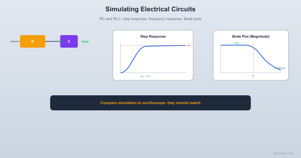
Generates step responses and Bode plots for RC and RLC circuits.
"""

import numpy as np
from scipy.integrate import solve_ivp
import matplotlib.pyplot as plt

# -------------------------------------------------------
# RC Circuit
# -------------------------------------------------------
def rc_step_response(R, C, V_step=1.0, t_end=None, n_points=1000):
    """
    Simulate step response of a series RC circuit.
    Returns time array and capacitor voltage array.
    """
    tau = R * C
    if t_end is None:
        t_end = 5 * tau  # 5 time constants

    def ode(t, y):
        Vc = y[0]
        dVc_dt = (V_step - Vc) / (R * C)
        return [dVc_dt]

    sol = solve_ivp(ode, [0, t_end], [0.0],
                    dense_output=True, max_step=t_end/500)

    t = np.linspace(0, t_end, n_points)
    Vc = sol.sol(t)[0]

    # Analytical solution for comparison
    Vc_analytical = V_step * (1 - np.exp(-t / tau))

    return t, Vc, Vc_analytical, tau

def rc_bode(R, C, f_min=1.0, f_max=1e6, n_points=500):
    """
    Compute Bode plot data for an RC low-pass filter.
    Returns frequency, magnitude (dB), and phase (degrees).
    """
    f = np.logspace(np.log10(f_min), np.log10(f_max), n_points)
    omega = 2 * np.pi * f
    H = 1.0 / (1.0 + 1j * omega * R * C)

    mag_db = 20 * np.log10(np.abs(H))
    phase_deg = np.degrees(np.angle(H))
    f_cutoff = 1.0 / (2 * np.pi * R * C)

    return f, mag_db, phase_deg, f_cutoff

# -------------------------------------------------------
# RLC Circuit
# -------------------------------------------------------
def rlc_step_response(R, L, C, V_step=1.0, t_end=None, n_points=1000):
    """
    Simulate step response of a series RLC circuit.
    Returns time, capacitor voltage, and inductor current.
    """
    omega_n = 1.0 / np.sqrt(L * C)
    zeta = R / 2.0 * np.sqrt(C / L)
    Q = 1.0 / (2.0 * zeta) if zeta > 0 else float('inf')

    if t_end is None:
        # Enough time to see the response settle
        if zeta < 1:
            # Underdamped: several oscillation periods
            omega_d = omega_n * np.sqrt(1 - zeta**2)
            t_end = max(10 * 2 * np.pi / omega_d, 20 / (zeta * omega_n))
        else:
            t_end = 10 / (zeta * omega_n)

    def ode(t, y):
        I_L = y[0]   # Inductor current
        V_C = y[1]   # Capacitor voltage
        dI_L_dt = (V_step - R * I_L - V_C) / L
        dV_C_dt = I_L / C
        return [dI_L_dt, dV_C_dt]

    sol = solve_ivp(ode, [0, t_end], [0.0, 0.0],
                    dense_output=True, max_step=t_end/2000)

    t = np.linspace(0, t_end, n_points)
    y = sol.sol(t)
    I_L = y[0]
    V_C = y[1]

    return t, V_C, I_L, omega_n, zeta, Q

def rlc_bode(R, L, C, f_min=1.0, f_max=1e6, n_points=500):
    """
    Compute Bode plot data for a series RLC circuit
    (voltage across capacitor / input voltage).
    """
    f = np.logspace(np.log10(f_min), np.log10(f_max), n_points)
    omega = 2 * np.pi * f

    # Transfer function: H(jw) = 1 / (1 - w^2*LC + jwRC)
    H = 1.0 / (1 - omega**2 * L * C + 1j * omega * R * C)

    mag_db = 20 * np.log10(np.abs(H))
    phase_deg = np.degrees(np.angle(H))

    f_resonant = 1.0 / (2 * np.pi * np.sqrt(L * C))

    return f, mag_db, phase_deg, f_resonant

# -------------------------------------------------------
# Analysis and Plotting
# -------------------------------------------------------
def analyze_rc(R, C):
    """Full analysis of an RC circuit."""
    print("=" * 55)
    print("  RC CIRCUIT ANALYSIS")
    print("=" * 55)

    tau = R * C
    f_c = 1.0 / (2 * np.pi * R * C)

    print(f"  R = {R:.1f} ohm")
    print(f"  C = {C*1e6:.2f} uF")
    print(f"  Time constant (tau) = {tau*1e3:.3f} ms")
    print(f"  Cutoff frequency    = {f_c:.1f} Hz")
    print(f"  5*tau (settling)    = {5*tau*1e3:.3f} ms")
    print("=" * 55)

    # Step response
    t, Vc_sim, Vc_analytical, _ = rc_step_response(R, C)

    # Bode plot
    f, mag, phase, _ = rc_bode(R, C, f_min=f_c/100, f_max=f_c*100)

    # Plot
    fig, axes = plt.subplots(2, 2, figsize=(12, 8))
    fig.suptitle(f"RC Circuit: R={R} ohm, C={C*1e6:.2f} uF", fontsize=13,
                 fontweight="bold")

    # Step response
    axes[0, 0].plot(t * 1e3, Vc_sim, "tab:blue", linewidth=2,
                     label="Simulation")
    axes[0, 0].plot(t * 1e3, Vc_analytical, "r--", linewidth=1.5,
                     label="Analytical", alpha=0.8)
    axes[0, 0].axhline(y=0.632, color="gray", linestyle=":", alpha=0.5)
    axes[0, 0].axvline(x=tau * 1e3, color="gray", linestyle=":", alpha=0.5,
                        label=f"tau = {tau*1e3:.3f} ms")
    axes[0, 0].set_xlabel("Time (ms)")
    axes[0, 0].set_ylabel("Capacitor Voltage (V)")
    axes[0, 0].set_title("Step Response")
    axes[0, 0].legend(fontsize=8)
    axes[0, 0].grid(True, alpha=0.3)

    # Error between simulation and analytical
    error = np.abs(Vc_sim - Vc_analytical)
    axes[0, 1].semilogy(t * 1e3, error + 1e-16, "tab:red", linewidth=1.5)
    axes[0, 1].set_xlabel("Time (ms)")
    axes[0, 1].set_ylabel("Absolute Error (V)")
    axes[0, 1].set_title("Simulation vs. Analytical Error")
    axes[0, 1].grid(True, alpha=0.3)

    # Bode magnitude
    axes[1, 0].semilogx(f, mag, "tab:blue", linewidth=2)
    axes[1, 0].axhline(y=-3, color="red", linestyle="--", alpha=0.7,
                        label="-3 dB")
    axes[1, 0].axvline(x=f_c, color="gray", linestyle=":", alpha=0.5,
                        label=f"fc = {f_c:.1f} Hz")
    axes[1, 0].set_xlabel("Frequency (Hz)")
    axes[1, 0].set_ylabel("Magnitude (dB)")
    axes[1, 0].set_title("Bode Plot: Magnitude")
    axes[1, 0].legend(fontsize=8)
    axes[1, 0].grid(True, alpha=0.3, which="both")

    # Bode phase
    axes[1, 1].semilogx(f, phase, "tab:orange", linewidth=2)
    axes[1, 1].axhline(y=-45, color="gray", linestyle=":", alpha=0.5,
                        label="-45 deg at fc")
    axes[1, 1].set_xlabel("Frequency (Hz)")
    axes[1, 1].set_ylabel("Phase (degrees)")
    axes[1, 1].set_title("Bode Plot: Phase")
    axes[1, 1].legend(fontsize=8)
    axes[1, 1].grid(True, alpha=0.3, which="both")

    plt.tight_layout()
    plt.savefig("rc_analysis.png", dpi=150, bbox_inches="tight")
    plt.show()
    print("Plot saved as rc_analysis.png\n")

def analyze_rlc(R, L, C):
    """Full analysis of an RLC circuit."""
    print("=" * 55)
    print("  RLC CIRCUIT ANALYSIS")
    print("=" * 55)

    omega_n = 1.0 / np.sqrt(L * C)
    f_n = omega_n / (2 * np.pi)
    zeta = R / 2.0 * np.sqrt(C / L)
    Q = 1.0 / (2.0 * zeta) if zeta > 0 else float('inf')

    if zeta < 1:
        damping_type = "Underdamped (will ring)"
    elif zeta == 1:
        damping_type = "Critically damped"
    else:
        damping_type = "Overdamped"

    print(f"  R = {R:.1f} ohm")
    print(f"  L = {L*1e3:.3f} mH")
    print(f"  C = {C*1e6:.2f} uF")
    print(f"  Natural frequency   = {f_n:.1f} Hz")
    print(f"  Damping ratio (z)   = {zeta:.4f}")
    print(f"  Quality factor (Q)  = {Q:.2f}")
    print(f"  Type: {damping_type}")
    print("=" * 55)

    # Step response
    t, V_C, I_L, _, _, _ = rlc_step_response(R, L, C)

    # Bode plot
    f, mag, phase, f_res = rlc_bode(R, L, C, f_min=f_n/100, f_max=f_n*100)

    # Plot
    fig, axes = plt.subplots(2, 2, figsize=(12, 8))
    fig.suptitle(
        f"RLC Circuit: R={R} ohm, L={L*1e3:.2f} mH, C={C*1e6:.2f} uF  "
        f"(zeta={zeta:.3f}, Q={Q:.1f})",
        fontsize=11, fontweight="bold")

    # Step response: voltage
    axes[0, 0].plot(t * 1e3, V_C, "tab:blue", linewidth=2)
    axes[0, 0].axhline(y=1.0, color="gray", linestyle="--", alpha=0.5,
                        label="Steady state")
    axes[0, 0].set_xlabel("Time (ms)")
    axes[0, 0].set_ylabel("Capacitor Voltage (V)")
    axes[0, 0].set_title("Step Response: Voltage")
    axes[0, 0].legend(fontsize=8)
    axes[0, 0].grid(True, alpha=0.3)

    # Step response: current
    axes[0, 1].plot(t * 1e3, I_L * 1e3, "tab:green", linewidth=2)
    axes[0, 1].set_xlabel("Time (ms)")
    axes[0, 1].set_ylabel("Inductor Current (mA)")
    axes[0, 1].set_title("Step Response: Current")
    axes[0, 1].grid(True, alpha=0.3)

    # Bode magnitude
    axes[1, 0].semilogx(f, mag, "tab:blue", linewidth=2)
    axes[1, 0].axhline(y=0, color="gray", linestyle="--", alpha=0.3)
    axes[1, 0].axvline(x=f_res, color="red", linestyle=":", alpha=0.7,
                        label=f"f_res = {f_res:.1f} Hz")
    axes[1, 0].set_xlabel("Frequency (Hz)")
    axes[1, 0].set_ylabel("Magnitude (dB)")
    axes[1, 0].set_title("Bode Plot: Magnitude")
    axes[1, 0].legend(fontsize=8)
    axes[1, 0].grid(True, alpha=0.3, which="both")

    # Bode phase
    axes[1, 1].semilogx(f, phase, "tab:orange", linewidth=2)
    axes[1, 1].axhline(y=-90, color="gray", linestyle=":", alpha=0.5)
    axes[1, 1].set_xlabel("Frequency (Hz)")
    axes[1, 1].set_ylabel("Phase (degrees)")
    axes[1, 1].set_title("Bode Plot: Phase")
    axes[1, 1].grid(True, alpha=0.3, which="both")

    plt.tight_layout()
    plt.savefig("rlc_analysis.png", dpi=150, bbox_inches="tight")
    plt.show()
    print("Plot saved as rlc_analysis.png\n")

# -------------------------------------------------------
# Main: run both analyses
# -------------------------------------------------------
if __name__ == "__main__":

    # RC circuit: 1k ohm, 10 uF (tau = 10 ms, fc = 15.9 Hz)
    analyze_rc(R=1000.0, C=10e-6)

    # RLC circuit: 100 ohm, 10 mH, 1 uF
    # This gives an underdamped response with visible ringing
    analyze_rlc(R=100.0, L=10e-3, C=1e-6)

    # Try an overdamped case too
    print("\n--- Overdamped RLC for comparison ---\n")
    analyze_rlc(R=1000.0, L=10e-3, C=1e-6)

Running the Analyzer

python circuit_analyzer.py

The script runs three analyses in sequence: one RC circuit and two RLC circuits (underdamped and overdamped). For each one, it prints the key parameters and generates a four-panel plot.

Expected output for the RC circuit:

=======================================================
  RC CIRCUIT ANALYSIS
=======================================================
  R = 1000.0 ohm
  C = 10.00 uF
  Time constant (tau) = 10.000 ms
  Cutoff frequency    = 15.9 Hz
  5*tau (settling)    = 50.000 ms
=======================================================

Comparing Simulation to Oscilloscope Measurements

The step response plot from the simulation shows exactly what you would see on an oscilloscope if you applied a voltage step to the circuit. Here is how to compare them:

On a real oscilloscope, you would:

Connect the function generator to the RC input, set to a square wave at a frequency much lower than
Probe the voltage across the capacitor
Measure the time to reach 63.2% of the step (that is )

In the simulation, the step response plot shows the same exponential curve. The error plot (top right) confirms that the simulation matches the exact analytical solution to within numerical precision (errors on the order of V).

Understanding the RLC Damping Ratio

The damping ratio determines the character of the circuit’s response. This concept appears again in Lesson 3 (mechanical systems) and Lesson 5 (control systems).

	Response Type	What You See
	Underdamped	Oscillation that decays over time
	Critically damped	Fastest settling, no overshoot
	Overdamped	Slow, no oscillation
	Undamped	Oscillation that never decays

For filter design, you typically want (Butterworth response), which gives a maximally flat passband with no resonance peak.

Experiments to Try

Butterworth Filter

For the RLC circuit, find the R value that gives (given L = 10 mH and C = 1 uF). Hint: rearrange the damping ratio formula to solve for R.

High-Pass Filter

Modify the code to plot the voltage across the resistor instead of the capacitor. This gives you a high-pass response. The transfer function changes to .

Notch Filter

A parallel RLC circuit can create a notch (band-reject) filter. Try modeling one and plotting its frequency response.

Component Tolerance

Real components have tolerances (typically 5% to 20%). Run the simulation 100 times with random R and C values drawn from a normal distribution around the nominal values. Plot all the Bode curves overlaid to see how tolerance affects the cutoff frequency.

Key Takeaways

RC circuits are first-order systems

One energy storage element (the capacitor) means one state variable and one time constant . The step response is a simple exponential.
RLC circuits are second-order systems

Two energy storage elements (inductor and capacitor) mean two state variables and the possibility of oscillation. The damping ratio controls whether it rings.
Time domain and frequency domain are two views of the same system

The step response tells you about transient behavior. The Bode plot tells you about steady-state frequency filtering. Both come from the same differential equations.
Simulation matches analytical results to numerical precision

For linear circuits, the analytical solution is known. The fact that the simulation matches it validates our approach for the nonlinear systems in later lessons where no closed-form solution exists.

Next Lesson

In the next lesson, we move from electrical to mechanical systems. You will model a spring-mass-damper system, sweep the damping ratio, and build a suspension tuner.

Mechanical System Dynamics →

Comments

Loading comments...