Spherical Cows and the Art of Model Building

Modified: Mar. 15, 2026

Published: Mar. 1, 2026

Become Contributor Expert Support

A farmer asks three experts how to increase milk production. The agronomist suggests better feed. The psychologist proposes stress reduction. The physicist begins: “Consider a spherical cow in a vacuum…” This old joke captures something real about how science works. The physicist is not being lazy. She is being strategic. She is asking: what details actually matter for this question, and what can I safely throw away? #AppliedMath #Modeling #Engineering

Why We Simplify

Every system in nature is, in some sense, infinitely complex. A cup of coffee cooling on your desk involves fluid convection, radiative heat transfer, evaporation from the surface, conduction through the ceramic, and the ambient air currents in the room. If you tried to model all of that from first principles, you would spend months and still miss something.

So you make a choice: what matters for my question?

If you just want to know roughly when the coffee will be cool enough to drink, most of those details are noise. You can treat the coffee as a single temperature that decreases toward room temperature at a rate proportional to the temperature difference. That is Newton’s law of cooling, and it is a “spherical cow” model. It ignores almost everything about the real physics. And it works remarkably well.

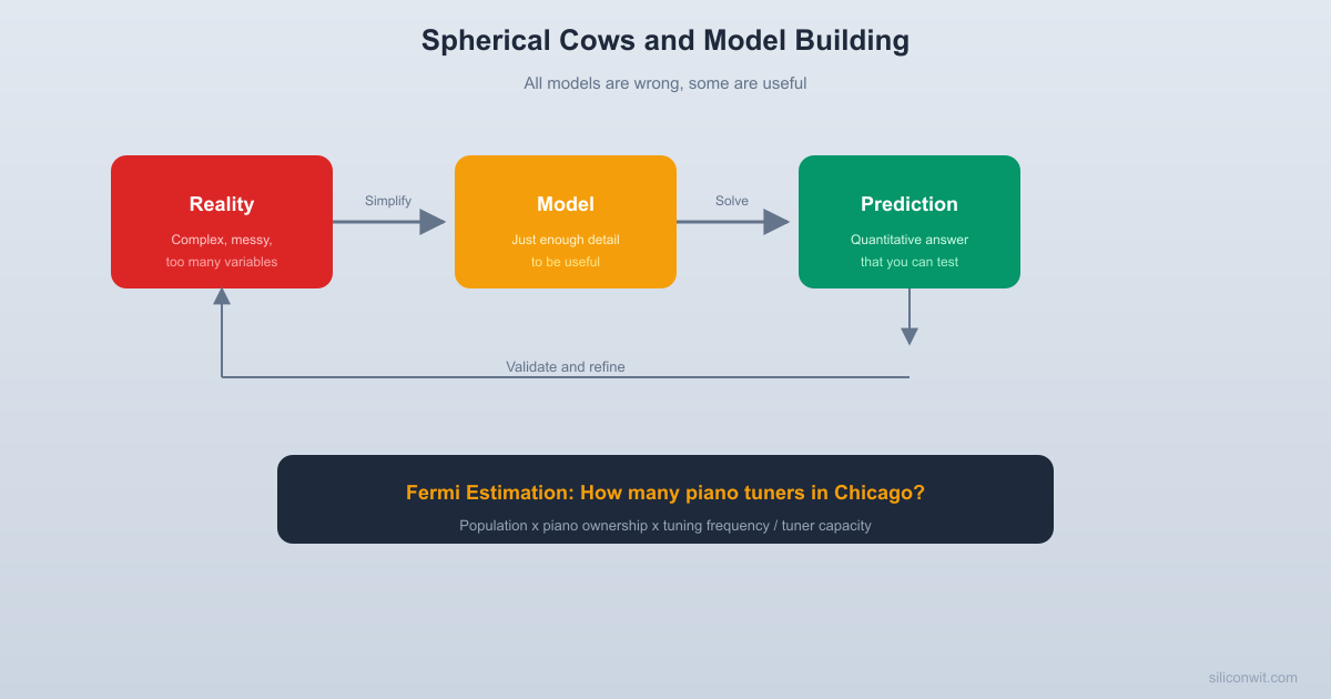
George Box, the statistician, said it best: “All models are wrong, but some are useful.”

The goal of modeling is not truth. It is usefulness. You are building a tool to answer a specific question, and the best tool is the simplest one that gives you a good enough answer.

From “Laws” to “Models”

Scientists used to talk about “laws of nature” as if they were absolute truths carved into the universe. Newton’s laws. Ohm’s law. The law of gravity. Today, we are more careful. Newton’s laws turned out to be a special case of Einstein’s relativity. Ohm’s law breaks down in semiconductors. Every “law” is really a model with a domain of validity, a range of conditions where it works well enough.

This is not a weakness. It is the entire point. A model that works for your conditions is all you need.

Fermi Estimation: The Art of the Quick Answer

Enrico Fermi was famous for asking questions that seemed impossible to answer: How many piano tuners are there in Chicago? He did not look this up. He estimated it, step by step, from things he already knew.

Here is how Fermi estimation works. You break the question into smaller questions you can estimate, multiply the pieces together, and arrive at an answer that is usually within a factor of 2 or 3 of the real number. That is often good enough.

Example: Piano Tuners in Chicago

1. How many people live in Chicago?

   About 2.7 million. Call it 3 million.

2. How many households?

   Average household size is about 2.5 people. So roughly 1.2 million households.

3. What fraction own a piano?

   Maybe 1 in 20 households. That gives 60,000 pianos.

4. How often is a piano tuned?

   About once a year.

5. How many pianos can one tuner service per day?

   A tuning takes about 2 hours including travel. So about 4 pianos per day, 5 days a week, 50 weeks a year. That is 1,000 pianos per tuner per year.

6. How many tuners?

   60,000 pianos divided by 1,000 per tuner = about 60 piano tuners.

The actual number is somewhere around 100. Our estimate of 60 is within a factor of 2. That is the power of Fermi estimation: you do not need precise data. You need the right structure.

Try these yourself: How much water does your city use per day? (Start with population, estimate liters per person for drinking, cooking, bathing, and toilets.) How many cars are on the highway right now? (Estimate the length of highway, average spacing between cars, and the number of lanes.) The same structure works every time.

Why Engineers Need This Skill

Before you spend a week building a simulation, spend five minutes estimating the answer. If your simulation says there should be 10,000 piano tuners, you know something went wrong. Fermi estimates provide sanity checks, and they train you to think in terms of orders of magnitude, which is how engineers think about most things.

The Modeling Cycle

Building a useful model is not a one-shot process. It is a cycle that you repeat until the model is good enough for your purpose.

1. Observe the system. What are the key variables? What is the output you care about? What drives it?

2. Simplify. Strip away everything that is not essential. Identify the dominant effects. Ignore the rest, for now.

3. Formulate. Write down the mathematical relationships. This might be an equation, a set of equations, or an algorithm.

4. Solve. Find the solution analytically (with algebra and calculus) or numerically (with a computer).

5. Validate. Compare your model’s predictions to real data or known results. Does it give reasonable answers?

6. Refine. If the model is not accurate enough, add back some of the complexity you removed. Then repeat.

The key insight is step 6: you only add complexity when the simple model fails. You never start with the most complex model. You start simple and build up.

Worked Example: A Cooling Cup of Coffee

Let us walk through the modeling cycle with a concrete problem.

The Question

You pour a cup of coffee at 90 degrees C. The room is at 22 degrees C. How long until the coffee reaches 50 degrees C (drinkable temperature)?

Step 1: Observe

The coffee is hot. The room is cooler. Heat flows from hot to cold. The coffee will cool down over time, approaching room temperature.

Step 2: Simplify

We treat the coffee as having a single uniform temperature (ignore the fact that the surface cools faster than the center). We ignore evaporation, radiation, and conduction through the mug. We assume the room temperature stays constant.

Step 3: Formulate

Newton’s law of cooling says that the rate of cooling is proportional to the temperature difference between the object and its surroundings:

where:

• is the coffee temperature
• is the room temperature
• is the cooling constant (depends on the mug, the amount of coffee, etc.)
• The minus sign means the temperature decreases when

Step 4: Solve

This is a separable first-order ODE. The solution is:

Plugging in and :

We need to find . If we measure the temperature after, say, 5 minutes and find it is 75 degrees C:

Now we can find when :

Step 5: Validate

Is 18 minutes reasonable? If you have ever left a cup of coffee on your desk, you know it cools noticeably in 5 minutes and is lukewarm in about 20 minutes. Our answer passes the sanity check.

Python Implementation

import numpy as np
import matplotlib.pyplot as plt

# Parameters
T_env = 22       # Room temperature (C)
T_0 = 90         # Initial coffee temperature (C)
k = 0.050        # Cooling constant (1/min)

# Time array
t = np.linspace(0, 60, 200)

# Newton's law of cooling
T = T_env + (T_0 - T_env) * np.exp(-k * t)

# Find when T = 50 C
t_drinkable = -np.log((50 - T_env) / (T_0 - T_env)) / k
print(f"Coffee reaches 50 C at t = {t_drinkable:.1f} minutes")

# Plot
plt.figure(figsize=(8, 5))
plt.plot(t, T, 'b-', linewidth=2)
plt.axhline(y=50, color='r', linestyle='--', label='Drinkable (50 C)')
plt.axhline(y=T_env, color='g', linestyle='--', label='Room temp (22 C)')
plt.axvline(x=t_drinkable, color='gray', linestyle=':', alpha=0.7)
plt.xlabel('Time (minutes)')
plt.ylabel('Temperature (C)')
plt.title('Coffee Cooling: Newton\'s Law of Cooling')
plt.legend()
plt.grid(True, alpha=0.3)
plt.show()

Worked Example: Estimating Battery Life from Duty Cycle

Here is a modeling problem every embedded engineer faces: how long will a battery last?

The Question

You have a sensor node powered by a 3000 mAh battery. The sensor wakes up every 60 seconds, takes a reading for 2 seconds (drawing 25 mA), then sleeps (drawing 10 uA). How many days will the battery last?

The Model

This is a weighted average problem. The device spends most of its time asleep, so the average current is dominated by the sleep current, plus a small contribution from the active periods.

      Active (2s)       Sleep (58s)
    |<---------->|<---------------------->|
    |  25 mA     |  0.010 mA              |
    |            |                        |
    |<----------- 60 second cycle ------->|

The duty cycle is (3.33%).

The average current is:

Battery life:

Step 6: Refine

That estimate assumes ideal conditions. In reality:

• Battery capacity decreases at low temperatures
• Self-discharge removes about 2-3% per month for lithium cells
• Voltage droop means the last 10-15% of capacity is often unusable
• The sensor might occasionally need longer active periods (transmitting data, retrying failed communications)

A conservative estimate would derate by 20-30%, giving roughly 100 to 120 days. That is still useful information for system design.

# Battery life calculation
capacity_mAh = 3000
active_time_s = 2
sleep_time_s = 58
cycle_time_s = active_time_s + sleep_time_s

I_active_mA = 25
I_sleep_mA = 0.010

duty_cycle = active_time_s / cycle_time_s
I_avg_mA = duty_cycle * I_active_mA + (1 - duty_cycle) * I_sleep_mA

life_hours = capacity_mAh / I_avg_mA
life_days = life_hours / 24

print(f"Duty cycle: {duty_cycle*100:.2f}%")
print(f"Average current: {I_avg_mA:.3f} mA")
print(f"Battery life: {life_hours:.0f} hours = {life_days:.0f} days")
print(f"Conservative (80%): {life_days*0.80:.0f} days")

When to Add Complexity

The hardest judgment call in modeling is knowing when to stop simplifying. Here are some guidelines.

The modeling cycle gives you a systematic way to navigate this. Start simple. Check against reality. Add complexity only where the simple model fails.

Common Model Types in Engineering

The Spherical Cow Philosophy

The spherical cow is not a joke about physicists being out of touch. It is a statement about the power of abstraction. When you simplify a cow to a sphere, you lose the legs, the spots, and the personality. But you gain the ability to calculate its thermal properties, its drag coefficient, and its moment of inertia. You trade detail for understanding.

Every equation in this course is a spherical cow of some kind. Newton’s law of cooling ignores convection currents. The ideal gas law ignores molecular interactions. Circuit models ignore quantum effects. They all work, within their domain of validity, because the simplifications they make do not matter for the questions they answer.

Learning to simplify, and knowing when your simplification breaks, is the most important skill in applied mathematics. It is not something you learn from a formula. It is something you develop through practice, by building models, testing them, and refining them until they work well enough.

The rest of this course will give you the mathematical tools for that process: calculus, linear algebra, complex numbers, differential equations, and more. But the philosophy starts here, with the spherical cow. Start simple. Check against reality. Add complexity only when you need it.