Simulating Signal Processing Pipelines

Modified: Mar. 15, 2026

Published: Mar. 7, 2026

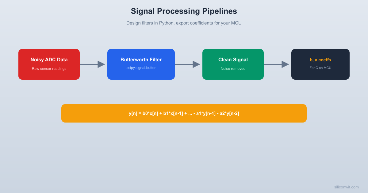
Raw ADC readings from a sensor are almost never clean enough to use directly. A temperature sensor on a vibrating motor, an accelerometer on a quadcopter, a current sense resistor next to a switching regulator: they all need filtering. The standard workflow is to design and validate the filter in Python where you can see every frequency component, then export the coefficients and implement the difference equation in C on your microcontroller. This lesson walks through that entire pipeline, from noisy signal to clean output to deployable code. #SignalProcessing #DigitalFilters #EmbeddedSystems

Digital Filter Fundamentals

The Core Idea

A digital filter is a mathematical operation on a sequence of numbers. It takes an input signal and produces an output signal by combining current and past values. Every digital filter can be described by its difference equation, its frequency response, and its impulse response. These are three views of the same object.

FIR vs IIR Filters

There are two families of digital filters:

Property	FIR (Finite Impulse Response)	IIR (Infinite Impulse Response)
Uses past outputs?	No	Yes
Stability	Always stable	Can be unstable
Phase response	Can be exactly linear	Nonlinear phase
Filter order for same sharpness	High (many taps)	Low (few coefficients)
Memory/computation	More	Less
Example	Moving average	Butterworth, Chebyshev

For embedded systems where memory and CPU cycles are tight, IIR filters are often preferred because they achieve sharp cutoffs with fewer coefficients.

The Difference Equation

Every IIR filter can be written as:

The coefficients multiply the input (feedforward path), and the coefficients multiply past outputs (feedback path). SciPy’s signal.butter gives you exactly these coefficients.

Moving Average Filter

The simplest FIR filter. It replaces each sample with the average of the surrounding samples:

The moving average is a low-pass filter. It smooths out high-frequency noise but has a very gentle rolloff, meaning it does not sharply separate signal from noise. Its frequency response has zeros at multiples of , where is the sample rate. For the mathematics behind frequency-domain analysis and the FFT, see Applied Mathematics: Fourier Analysis and the Frequency Domain.

When to use it: Quick noise reduction where sharp cutoff is not critical. Very easy to implement on any MCU: just a circular buffer and a running sum.

Butterworth Filter

The Butterworth filter is the workhorse of signal processing. It has the flattest possible passband (no ripple), a smooth monotonic rolloff, and predictable phase behavior. It is an IIR filter defined by two parameters:

Cutoff frequency : the frequency at which the gain drops to dB (about 70.7% of the passband amplitude)
Order : higher order means sharper rolloff (steeper transition from pass to stop) but more computation and more phase distortion

A 4th-order Butterworth rolling off at 20 dB/decade per order gives 80 dB/decade of attenuation. For most sensor filtering applications, 2nd to 4th order is sufficient.

Designing with SciPy

scipy.signal.butter(N, Wn, btype, fs)

N: filter order
Wn: cutoff frequency in Hz (when fs is specified)
btype: ‘low’, ‘high’, ‘bandpass’, ‘bandstop’
fs: sample rate in Hz

This returns (b, a) coefficient arrays that you can use directly in scipy.signal.lfilter or implement as a difference equation in C.

Resampling and Decimation

Sometimes your ADC runs at a much higher rate than you need. A 12-bit ADC sampling at 10 kHz feeding a temperature control loop that updates at 100 Hz has 100x more data than necessary. Decimation reduces the sample rate by keeping every -th sample, but you must low-pass filter first to prevent aliasing.

Original signal:  [x0, x1, x2, x3, x4, x5, x6, x7, x8, x9, ...]
                         |              |              |
Anti-alias filter:  Low-pass at fs/(2*M) Hz
                         |              |              |
Decimate by M=3:  [x0,             x3,             x6,         ...]

The anti-aliasing filter prevents high-frequency content above the new Nyquist frequency from folding back into the signal as artifacts.

Project: Noise Filter Designer

What You Will Build

A complete filter design tool that generates noisy sensor data (or loads a CSV), designs a Butterworth low-pass filter, applies it, and visualizes the before and after in both time domain and frequency domain. The tool also outputs the filter coefficients in a format you can copy directly into a C implementation for your microcontroller.

Complete Runnable Code

import numpy as np
import matplotlib.pyplot as plt
from scipy import signal

# ============================================================
# Noise Filter Designer for Sensor Data
# ============================================================
# Design filters in Python, export coefficients for embedded C.

np.random.seed(42)

# --- Signal parameters ---
fs = 1000.0        # Sample rate (Hz) - typical ADC rate
duration = 2.0     # seconds
t = np.arange(0, duration, 1.0 / fs)
N = len(t)

# --- Generate a realistic sensor signal ---
# Slow-changing "true" signal: temperature ramp + small oscillation
true_signal = 25.0 + 3.0 * (t / duration) + 0.5 * np.sin(2 * np.pi * 2 * t)

# Add realistic noise components:
# 1. White noise from ADC quantization and thermal noise
white_noise = 0.8 * np.random.randn(N)

# 2. 50/60 Hz power line interference
power_line_50 = 0.6 * np.sin(2 * np.pi * 50 * t)
power_line_60 = 0.3 * np.sin(2 * np.pi * 60 * t)

# 3. High-frequency switching noise (from a DC-DC converter nearby)
switching_noise = 0.4 * np.sin(2 * np.pi * 200 * t + np.random.uniform(0, 2*np.pi))

# Combined noisy signal (what the ADC actually reads)
noisy_signal = true_signal + white_noise + power_line_50 + power_line_60 + switching_noise

# ============================================================
# Filter 1: Moving Average
# ============================================================
def moving_average(x, window_size):
    """Simple moving average filter."""
    kernel = np.ones(window_size) / window_size
    # Use 'valid' mode and pad to maintain length
    filtered = np.convolve(x, kernel, mode='same')
    return filtered

ma_window = 50  # 50 samples at 1 kHz = 50 ms window
ma_filtered = moving_average(noisy_signal, ma_window)

# ============================================================
# Filter 2: Butterworth Low-Pass
# ============================================================
# Design: we want to keep signals below 10 Hz (our sensor changes slowly)
# and remove everything above (noise, power line, switching)
cutoff_hz = 10.0
filter_order = 4

b, a = signal.butter(filter_order, cutoff_hz, btype='low', fs=fs)
butter_filtered = signal.filtfilt(b, a, noisy_signal)  # zero-phase filtering

# Also apply with lfilter (causal, as it would run on an MCU)
butter_causal = signal.lfilter(b, a, noisy_signal)

# ============================================================
# Filter 3: Higher-order Butterworth for comparison
# ============================================================
b8, a8 = signal.butter(8, cutoff_hz, btype='low', fs=fs)
butter8_filtered = signal.filtfilt(b8, a8, noisy_signal)

# ============================================================
# Frequency domain analysis
# ============================================================
def compute_spectrum(x, fs):
    """Compute single-sided amplitude spectrum."""
    n = len(x)
    freqs = np.fft.rfftfreq(n, 1.0 / fs)
    magnitude = 2.0 / n * np.abs(np.fft.rfft(x))
    return freqs, magnitude

freqs_noisy, mag_noisy = compute_spectrum(noisy_signal, fs)
freqs_butter, mag_butter = compute_spectrum(butter_filtered, fs)

# Filter frequency response
w, h = signal.freqz(b, a, worN=2048, fs=fs)
w8, h8 = signal.freqz(b8, a8, worN=2048, fs=fs)

# ============================================================
# Compute errors
# ============================================================
rmse_noisy = np.sqrt(np.mean((noisy_signal - true_signal) ** 2))
rmse_ma = np.sqrt(np.mean((ma_filtered - true_signal) ** 2))
rmse_butter = np.sqrt(np.mean((butter_filtered - true_signal) ** 2))
rmse_butter8 = np.sqrt(np.mean((butter8_filtered - true_signal) ** 2))

print("=" * 60)
print("  Noise Filter Designer: Results")
print("=" * 60)
print(f"  Sample rate:          {fs:.0f} Hz")
print(f"  Signal duration:      {duration:.1f} s")
print(f"  Butterworth cutoff:   {cutoff_hz:.0f} Hz, order {filter_order}")
print("-" * 60)
print(f"  Raw noisy signal     RMSE: {rmse_noisy:.4f}")
print(f"  Moving average (M={ma_window:d})  RMSE: {rmse_ma:.4f}")
print(f"  Butterworth order 4  RMSE: {rmse_butter:.4f}")
print(f"  Butterworth order 8  RMSE: {rmse_butter8:.4f}")
print("=" * 60)

# ============================================================
# Export coefficients for C implementation
# ============================================================
print("\n--- C-ready filter coefficients ---")
print(f"// Butterworth low-pass, order {filter_order}, cutoff {cutoff_hz} Hz, fs {fs:.0f} Hz")
print(f"// Generated by scipy.signal.butter")
print(f"#define FILTER_ORDER {filter_order}")
print(f"#define NUM_B_COEFFS {len(b)}")
print(f"#define NUM_A_COEFFS {len(a)}")
print()
b_str = ", ".join(f"{coeff:.15e}" for coeff in b)
a_str = ", ".join(f"{coeff:.15e}" for coeff in a)
print(f"const double b[] = {{{b_str}}};")
print(f"const double a[] = {{{a_str}}};")
print()
print("// Difference equation implementation:")
print("// y[n] = b[0]*x[n] + b[1]*x[n-1] + ... + b[M]*x[n-M]")
print("//       - a[1]*y[n-1] - a[2]*y[n-2] - ... - a[N]*y[n-N]")
print("// (a[0] is always 1.0 for normalized coefficients)")

# ============================================================
# Decimation example
# ============================================================
decim_factor = 10  # Reduce from 1000 Hz to 100 Hz

# Anti-aliasing filter: cutoff at new Nyquist (50 Hz)
b_aa, a_aa = signal.butter(4, (fs / decim_factor) / 2.0 * 0.8, btype='low', fs=fs)
anti_aliased = signal.filtfilt(b_aa, a_aa, noisy_signal)
decimated = anti_aliased[::decim_factor]
t_decimated = t[::decim_factor]

print(f"\n--- Decimation ---")
print(f"  Original:  {N} samples at {fs:.0f} Hz")
print(f"  Decimated: {len(decimated)} samples at {fs/decim_factor:.0f} Hz")

# ============================================================
# Plot everything
# ============================================================
fig, axes = plt.subplots(4, 1, figsize=(12, 16))

# Plot 1: Time domain comparison
ax = axes[0]
ax.plot(t, noisy_signal, 'gray', linewidth=0.5, alpha=0.5, label='Noisy signal')
ax.plot(t, true_signal, 'k-', linewidth=2, label='True signal')
ax.plot(t, ma_filtered, 'b-', linewidth=1.5, label=f'Moving avg (M={ma_window})')
ax.plot(t, butter_filtered, 'r-', linewidth=1.5, label=f'Butterworth (n={filter_order})')
ax.set_ylabel('Amplitude')
ax.set_title('Time Domain: Noisy vs Filtered')
ax.legend(loc='upper left', fontsize=9)
ax.grid(True, alpha=0.3)
ax.set_xlim([0, 0.5])  # Zoom into first 0.5s for detail

# Plot 2: Frequency domain before and after
ax = axes[1]
ax.semilogy(freqs_noisy, mag_noisy, 'gray', alpha=0.7, label='Noisy signal spectrum')
ax.semilogy(freqs_butter, mag_butter, 'r-', linewidth=1.5, label='After Butterworth')
ax.axvline(x=50, color='orange', linestyle=':', alpha=0.7, label='50 Hz power line')
ax.axvline(x=60, color='orange', linestyle='--', alpha=0.7, label='60 Hz power line')
ax.axvline(x=cutoff_hz, color='green', linestyle='-', alpha=0.7, label=f'Cutoff: {cutoff_hz} Hz')
ax.set_xlabel('Frequency (Hz)')
ax.set_ylabel('Magnitude')
ax.set_title('Frequency Domain: Noise Components Removed')
ax.legend(loc='upper right', fontsize=9)
ax.grid(True, alpha=0.3)
ax.set_xlim([0, 300])

# Plot 3: Filter frequency response
ax = axes[2]
ax.plot(w, 20 * np.log10(np.abs(h) + 1e-15), 'r-', linewidth=2,
        label=f'Order {filter_order}')
ax.plot(w8, 20 * np.log10(np.abs(h8) + 1e-15), 'b--', linewidth=2,
        label='Order 8')
ax.axvline(x=cutoff_hz, color='green', linestyle=':', label=f'Cutoff: {cutoff_hz} Hz')
ax.axhline(y=-3, color='gray', linestyle=':', alpha=0.5, label='-3 dB')
ax.set_xlabel('Frequency (Hz)')
ax.set_ylabel('Gain (dB)')
ax.set_title('Butterworth Filter Frequency Response')
ax.legend(loc='lower left', fontsize=9)
ax.grid(True, alpha=0.3)
ax.set_xlim([0, 100])
ax.set_ylim([-80, 5])

# Plot 4: Causal vs zero-phase and decimation
ax = axes[3]
ax.plot(t, true_signal, 'k-', linewidth=2, label='True signal')
ax.plot(t, butter_causal, 'b-', linewidth=1.2, alpha=0.7,
        label='Causal (lfilter, has delay)')
ax.plot(t, butter_filtered, 'r-', linewidth=1.2,
        label='Zero-phase (filtfilt, no delay)')
ax.plot(t_decimated, decimated, 'go', markersize=4,
        label=f'Decimated ({fs/decim_factor:.0f} Hz)')
ax.set_xlabel('Time (s)')
ax.set_ylabel('Amplitude')
ax.set_title('Causal vs Zero-Phase Filtering, and Decimation')
ax.legend(loc='upper left', fontsize=9)
ax.grid(True, alpha=0.3)
ax.set_xlim([0, 0.5])

plt.tight_layout()
plt.savefig('noise_filter_designer.png', dpi=150, bbox_inches='tight')
plt.show()
print("\nPlot saved: noise_filter_designer.png")

Understanding the Output

Time domain plot shows the noisy ADC signal (gray), the true underlying signal (black), and two filtered versions. The Butterworth filter tracks the true signal closely while removing almost all noise. The moving average also helps but has more residual ripple.
Frequency domain plot reveals the noise components: peaks at 50 Hz and 60 Hz from power line interference, a bump around 200 Hz from switching noise, and broadband white noise everywhere. After Butterworth filtering, everything above 10 Hz is gone.
Filter response plot compares the 4th-order and 8th-order Butterworth frequency responses. The 4th-order rolls off at 80 dB/decade; the 8th-order at 160 dB/decade. Higher order means sharper cutoff but more computation and more phase distortion.
Causal vs zero-phase plot demonstrates a critical distinction. The lfilter (causal) output has a time delay because the filter can only use past and present samples, exactly as it would run on a microcontroller. The filtfilt (zero-phase) output has no delay because it processes the signal forward and backward, but this is only possible offline.

From Python to C: Implementing on a Microcontroller

The filter coefficients printed by the code are directly usable in C. Here is the general structure for a direct-form IIR filter on an MCU:

// IIR filter implementation for embedded systems
// Paste the b[] and a[] arrays from Python output

static double x_buf[NUM_B_COEFFS] = {0};  // input history
static double y_buf[NUM_A_COEFFS] = {0};  // output history

double iir_filter(double x_new) {
    // Shift input buffer
    for (int i = NUM_B_COEFFS - 1; i > 0; i--)
        x_buf[i] = x_buf[i - 1];
    x_buf[0] = x_new;

    // Shift output buffer
    for (int i = NUM_A_COEFFS - 1; i > 0; i--)
        y_buf[i] = y_buf[i - 1];

    // Compute new output
    double y_new = 0.0;
    for (int i = 0; i < NUM_B_COEFFS; i++)
        y_new += b[i] * x_buf[i];
    for (int i = 1; i < NUM_A_COEFFS; i++)
        y_new -= a[i] * y_buf[i];

    y_buf[0] = y_new;
    return y_new;
}

Call iir_filter() once per ADC sample in your timer interrupt. The output is the filtered value. This is the difference equation running in real time.

Important: Causal Filtering on MCUs

On a microcontroller, you can only use causal filtering (lfilter equivalent). The filter only has access to current and past samples, never future ones. This means there will be a small phase delay in the output. For most control and measurement applications, this delay is acceptable. If it matters, you can compensate for it in your control loop or reduce the filter order.

Filter Design Guidelines

Sensor Application	Suggested Cutoff	Order	Notes
Temperature (slow)	1 to 5 Hz	2	Thermal time constants are slow
Pressure sensor	5 to 20 Hz	2 to 4	Depends on measurement speed
Accelerometer (tilt)	5 to 10 Hz	4	Remove vibration, keep gravity
Current sensing	50 to 200 Hz	4	Keep dynamics, remove switching noise
Audio preprocessing	20 to 4000 Hz	4 to 6	Bandpass for voice
Vibration monitoring	Application specific	4 to 8	Often bandpass around resonance

Exercises

Notch filter. Design a bandstop (notch) filter to remove only the 50 Hz power line interference without affecting the rest of the signal. Use signal.iirnotch. Compare the result with the low-pass approach.
FIR comparison. Design a 50-tap FIR filter using signal.firwin with the same 10 Hz cutoff. Compare the frequency response, group delay, and RMSE against the 4th-order Butterworth. How many FIR taps do you need to match the Butterworth’s sharpness?
Real data. Record ADC data from an actual sensor (or download a noisy sensor dataset from the web). Load it as a CSV, apply the Butterworth filter, and visualize. How do you choose the cutoff frequency when you do not know the true signal?
Fixed-point coefficients. Convert the floating-point b and a coefficients to Q15 fixed-point format (multiply by 32768 and round to integers). Implement the filter using integer arithmetic only. Compare the fixed-point output to the floating-point output. How much error does quantization introduce?
Cascaded second-order sections. For filter orders above 4, direct form implementation can be numerically unstable. Use signal.butter(..., output='sos') to get second-order sections. Implement the cascade and compare stability.

References

Oppenheim, A. V. and Schafer, R. W. (2009). Discrete-Time Signal Processing. Prentice Hall. The standard DSP textbook.
Smith, S. W. (1997). The Scientist and Engineer’s Guide to Digital Signal Processing. Free online: dspguide.com. Excellent intuitive explanations.
SciPy Signal Processing documentation: docs.scipy.org/doc/scipy/reference/signal.html
Texas Instruments Application Note SLAA447. IIR Filter Design on the MSP430. Practical embedded implementation guide.

Comments

Loading comments...