Sensor Fusion and State Estimation

Modified: Mar. 15, 2026

Published: Mar. 6, 2026

Become Contributor Expert Support

Every drone, phone, robot, and VR headset estimates its orientation dozens of times per second. The raw sensor data is never good enough on its own. Accelerometers measure gravity (plus every bump and vibration), and gyroscopes measure angular rate (but accumulate drift over time). Sensor fusion is the set of algorithms that merge these imperfect measurements into a single, reliable state estimate. This lesson builds both a complementary filter and a Kalman filter from scratch, then compares them side by side on simulated IMU data. #SensorFusion #KalmanFilter #IMU

The Problem with Single Sensors

Accelerometer Angle Estimation

When the sensor is stationary (or moving at constant velocity), the only acceleration it measures is gravity. The tilt angle around one axis is:

This works perfectly on a desk. On a moving robot or a vibrating motor mount, the signal looks like a noisy mess.

Gyroscope Angle Estimation

The gyroscope outputs angular rate in degrees per second. To get angle, you integrate:

This is smooth and responsive, but each small measurement error accumulates. After a few minutes, the estimated angle can be off by tens of degrees.

Sensor Fusion Block Diagram

                    +-----------------+
  Accelerometer --->| Low-pass filter |---+
  (noisy, stable)   +-----------------+   |
                                          +--> Fused angle estimate
  Gyroscope ------->| High-pass filter|---+
  (smooth, drifts)  +-----------------+

  Complementary filter:
    angle = alpha * (angle + gyro * dt) + (1 - alpha) * accel_angle

  Kalman filter:
    Predict:  x_hat = A * x_hat + B * u
              P     = A * P * A^T + Q
    Update:   K     = P * H^T * (H * P * H^T + R)^(-1)
              x_hat = x_hat + K * (z - H * x_hat)
              P     = (I - K * H) * P

The Complementary Filter

The complementary filter is elegant in its simplicity. It is a weighted blend of two estimates: trust the gyroscope for short-term changes (high-frequency), and trust the accelerometer for long-term stability (low-frequency). A single parameter (typically 0.95 to 0.98) controls the tradeoff:

When , you trust the gyroscope 98% and the accelerometer 2% at each time step. The gyroscope provides the fast response, while the accelerometer slowly corrects any drift. This filter runs on any microcontroller with a single multiply-add operation per sample.

Choosing Alpha

The time constant of the complementary filter is:

For and s (100 Hz), s. Signals faster than this come mostly from the gyroscope; slower signals come from the accelerometer. If you increase , drift correction becomes slower but the output is smoother. If you decrease , drift corrects faster but accelerometer noise leaks through.

The Kalman Filter

The Kalman filter is the optimal linear estimator for Gaussian noise. Instead of a fixed weighting like the complementary filter, it computes a time-varying gain based on how much it trusts the model versus the measurement. The core idea has two steps.

Predict Step

Given a state vector (containing angle and gyro bias) and a process model:

Here is the state transition matrix, maps the control input (gyro rate), is the error covariance, and is the process noise covariance.

Update Step

When a measurement (accelerometer angle) arrives:

The Kalman gain automatically adjusts: when the measurement is trustworthy ( is small), the gain is large and the filter follows the measurement closely. When the measurement is noisy ( is large), the gain is small and the filter relies on the model prediction. For the matrix algebra behind these operations, see Applied Mathematics: Linear Algebra, Vectors, and Matrices.

State Vector for IMU Fusion

For a 1-axis IMU fusion problem, the state vector is:

where is the angle and is the gyroscope bias (the drift rate). The filter estimates both simultaneously. This is a key advantage over the complementary filter: the Kalman filter explicitly models and corrects for gyro bias.

Project: IMU Orientation Estimator

Complete Runnable Code

import numpy as np
import matplotlib.pyplot as plt

# ============================================================
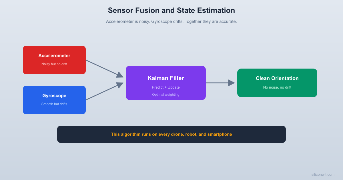
# IMU Orientation Estimator: Complementary + Kalman Filter
# ============================================================
# Simulates accelerometer and gyroscope data with realistic
# noise, then fuses them using two different algorithms.

np.random.seed(42)

# --- Simulation parameters ---
dt = 0.01              # 100 Hz sample rate
t_end = 60.0           # 60 seconds of data
t = np.arange(0, t_end, dt)
N = len(t)

# --- True angle trajectory ---
# Slow sinusoidal motion (like a robot arm or gimbal)
true_angle = 30.0 * np.sin(0.2 * t) + 10.0 * np.sin(0.05 * t)
true_rate = np.gradient(true_angle, dt)  # true angular rate (deg/s)

# --- Simulated accelerometer ---
# Good for static angle, but noisy and affected by vibrations
accel_noise_std = 3.0  # degrees
vibration_noise = 5.0 * np.sin(50 * t) * np.exp(-0.05 * t)  # decaying vibration
accel_angle = true_angle + accel_noise_std * np.random.randn(N) + vibration_noise

# Add occasional impulse disturbances (bumps)
bump_indices = np.random.choice(N, size=20, replace=False)
accel_angle[bump_indices] += np.random.uniform(-15, 15, size=20)

# --- Simulated gyroscope ---
# Smooth but drifts over time
gyro_noise_std = 0.3   # deg/s
gyro_bias_rate = 0.02  # deg/s drift accumulation rate
gyro_bias = np.cumsum(gyro_bias_rate * dt * np.random.randn(N))
gyro_rate = true_rate + gyro_noise_std * np.random.randn(N) + gyro_bias

# --- Raw gyro integration (to show drift) ---
gyro_angle = np.zeros(N)
gyro_angle[0] = accel_angle[0]
for i in range(1, N):
    gyro_angle[i] = gyro_angle[i - 1] + gyro_rate[i] * dt

# ============================================================
# Complementary Filter
# ============================================================
def complementary_filter(accel_angle, gyro_rate, dt, alpha=0.98):
    """
    Fuse accelerometer angle and gyroscope rate.
    alpha: weight for gyroscope (0.95 to 0.99 typical).
    """
    n = len(accel_angle)
    angle = np.zeros(n)
    angle[0] = accel_angle[0]

    for i in range(1, n):
        # Gyro prediction + accel correction
        angle[i] = alpha * (angle[i - 1] + gyro_rate[i] * dt) \
                   + (1 - alpha) * accel_angle[i]

    return angle

# ============================================================
# Kalman Filter for IMU Fusion
# ============================================================
def kalman_filter_imu(accel_angle, gyro_rate, dt,
                      Q_angle=0.001, Q_bias=0.003, R_measure=3.0):
    """
    2-state Kalman filter: estimates angle and gyro bias.

    State: x = [angle, bias]^T
    Prediction:  angle_new = angle + (gyro - bias) * dt
                 bias_new  = bias
    Measurement: z = accel_angle

    Q_angle:   process noise for angle state
    Q_bias:    process noise for bias state
    R_measure: measurement noise (accelerometer variance)
    """
    n = len(accel_angle)
    angle_est = np.zeros(n)
    bias_est = np.zeros(n)

    # Initial state
    angle_est[0] = accel_angle[0]
    bias_est[0] = 0.0

    # Error covariance matrix P (2x2)
    P = np.array([[1.0, 0.0],
                  [0.0, 1.0]])

    # Process noise covariance
    Q = np.array([[Q_angle, 0.0],
                  [0.0, Q_bias]])

    # Measurement matrix: we only measure angle
    H = np.array([[1.0, 0.0]])
    R = np.array([[R_measure]])

    for i in range(1, n):
        # --- Predict ---
        # State prediction
        rate = gyro_rate[i] - bias_est[i - 1]
        angle_pred = angle_est[i - 1] + rate * dt
        bias_pred = bias_est[i - 1]

        # Covariance prediction
        # A = [[1, -dt], [0, 1]]
        A = np.array([[1.0, -dt],
                      [0.0, 1.0]])
        P = A @ P @ A.T + Q

        # --- Update ---
        # Innovation (measurement residual)
        z = accel_angle[i]
        y = z - angle_pred  # H @ x_pred = angle_pred

        # Innovation covariance
        S = P[0, 0] + R_measure

        # Kalman gain (2x1)
        K = np.array([[P[0, 0] / S],
                      [P[1, 0] / S]])

        # State update
        angle_est[i] = angle_pred + K[0, 0] * y
        bias_est[i] = bias_pred + K[1, 0] * y

        # Covariance update
        I_KH = np.array([[1.0 - K[0, 0], 0.0],
                         [-K[1, 0], 1.0]])
        P = I_KH @ P

    return angle_est, bias_est

# ============================================================
# Run both filters
# ============================================================
comp_angle = complementary_filter(accel_angle, gyro_rate, dt, alpha=0.98)
kalman_angle, kalman_bias = kalman_filter_imu(
    accel_angle, gyro_rate, dt,
    Q_angle=0.001, Q_bias=0.003, R_measure=4.0
)

# ============================================================
# Compute errors
# ============================================================
accel_rmse = np.sqrt(np.mean((accel_angle - true_angle) ** 2))
gyro_rmse = np.sqrt(np.mean((gyro_angle - true_angle) ** 2))
comp_rmse = np.sqrt(np.mean((comp_angle - true_angle) ** 2))
kalman_rmse = np.sqrt(np.mean((kalman_angle - true_angle) ** 2))

print("=" * 55)
print("  IMU Orientation Estimation: Error Comparison")
print("=" * 55)
print(f"  Raw Accelerometer  RMSE: {accel_rmse:8.3f} deg")
print(f"  Raw Gyro (integrated)  : {gyro_rmse:8.3f} deg")
print(f"  Complementary Filter   : {comp_rmse:8.3f} deg")
print(f"  Kalman Filter          : {kalman_rmse:8.3f} deg")
print("=" * 55)
print(f"\n  Complementary filter is {accel_rmse / comp_rmse:.1f}x better than raw accel")
print(f"  Kalman filter is {accel_rmse / kalman_rmse:.1f}x better than raw accel")

# ============================================================
# Plot results
# ============================================================
fig, axes = plt.subplots(4, 1, figsize=(12, 14), sharex=True)

# Plot 1: Raw sensor data vs truth
ax = axes[0]
ax.plot(t, true_angle, 'k-', linewidth=2, label='True angle')
ax.plot(t, accel_angle, 'r.', markersize=1, alpha=0.3, label=f'Accel (RMSE={accel_rmse:.1f})')
ax.plot(t, gyro_angle, 'b-', alpha=0.5, label=f'Gyro integrated (RMSE={gyro_rmse:.1f})')
ax.set_ylabel('Angle (deg)')
ax.set_title('Raw Sensor Data: Neither Is Good Enough')
ax.legend(loc='upper right', fontsize=9)
ax.grid(True, alpha=0.3)

# Plot 2: Complementary filter
ax = axes[1]
ax.plot(t, true_angle, 'k-', linewidth=2, label='True angle')
ax.plot(t, comp_angle, 'g-', linewidth=1.5, label=f'Complementary (RMSE={comp_rmse:.2f})')
ax.set_ylabel('Angle (deg)')
ax.set_title('Complementary Filter: Simple but Effective')
ax.legend(loc='upper right', fontsize=9)
ax.grid(True, alpha=0.3)

# Plot 3: Kalman filter
ax = axes[2]
ax.plot(t, true_angle, 'k-', linewidth=2, label='True angle')
ax.plot(t, kalman_angle, 'm-', linewidth=1.5, label=f'Kalman (RMSE={kalman_rmse:.2f})')
ax.set_ylabel('Angle (deg)')
ax.set_title('Kalman Filter: Optimal Estimation')
ax.legend(loc='upper right', fontsize=9)
ax.grid(True, alpha=0.3)

# Plot 4: Estimated gyro bias
ax = axes[3]
ax.plot(t, gyro_bias, 'b-', linewidth=1.5, label='True gyro bias')
ax.plot(t, kalman_bias, 'r--', linewidth=1.5, label='Kalman bias estimate')
ax.set_xlabel('Time (s)')
ax.set_ylabel('Bias (deg/s)')
ax.set_title('Kalman Filter Tracks Gyroscope Bias')
ax.legend(loc='upper right', fontsize=9)
ax.grid(True, alpha=0.3)

plt.tight_layout()
plt.savefig('imu_sensor_fusion.png', dpi=150, bbox_inches='tight')
plt.show()
print("\nPlot saved: imu_sensor_fusion.png")

What the Code Does

1. Generates a realistic true trajectory. A slow sinusoidal angle profile that mimics a robot arm or gimbal moving back and forth.

2. Simulates accelerometer data. Adds Gaussian noise, decaying vibration, and random impulse bumps to the true angle. This represents what a real MEMS accelerometer produces on a moving platform.

3. Simulates gyroscope data. Adds small Gaussian noise to the true rate, plus a slowly accumulating bias that represents MEMS gyro drift. Integrating this signal produces an angle that diverges from truth over time.

4. Applies the complementary filter. A single line of code per sample blends the gyro prediction with the accel measurement. The weighting trusts the gyroscope for fast motion and the accelerometer for slow drift correction.

5. Applies the Kalman filter. A two-state filter (angle + bias) that predicts using the gyroscope, then corrects using the accelerometer. It automatically estimates the gyroscope bias and subtracts it from future predictions.

6. Plots all four estimates. The comparison makes the improvement immediately visible: raw sensors are noisy or drifting, while fused estimates track the true angle closely.

Tuning the Filters

Complementary Filter Tuning

The only knob is . Here is what happens when you change it:

Kalman Filter Tuning

The Kalman filter has three tuning parameters:

The ratio determines how aggressive the filter is. A large makes it responsive but noisier. A small makes it smooth but slower to correct.

When to Use Which Filter

Extending to 3D: The Full IMU Problem

The 1-axis problem in this lesson extends directly to 3D. A full IMU produces three accelerometer axes and three gyroscope axes. The state vector expands to include roll, pitch, and yaw (or quaternion components), each with its own bias term. The filter structure is identical; only the matrix dimensions change.

For roll and pitch, the accelerometer provides a gravity reference. For yaw, there is no gravity reference (gravity is parallel to the yaw axis), so a magnetometer is typically added as a third sensor. This is why most IMU modules include a magnetometer and are called 9-DOF (9 degrees of freedom): 3 accel + 3 gyro + 3 mag.

The same fusion principles apply. The Kalman filter simply grows from a 2-state system to a 6-state or 7-state system. Libraries like Madgwick and Mahony implement efficient versions of this for embedded platforms.

Practical Considerations

Sample Rate Matters

The complementary filter’s effective time constant depends on the sample rate. At 100 Hz with , the time constant is about 0.5 seconds. At 50 Hz with the same , the time constant doubles. When you change sample rate, you should re-tune .

Numerical Stability

The Kalman filter’s covariance matrix can become non-positive-definite due to floating-point errors over thousands of iterations. On embedded systems, the Joseph form of the covariance update is more numerically stable:

Real Sensor Data

The simulation in this lesson uses noise parameters typical of low-cost MEMS sensors (MPU6050, BMI160, LSM6DS3). If you have a real IMU, you can log data over USB or SD card, load the CSV into Python, and run the same filters. The tuning process is the same: adjust Q, R, and alpha until the output looks clean and responsive.

Exercises

1. Alpha sweep. Run the complementary filter with values from 0.80 to 0.99 in steps of 0.01. Plot RMSE versus . Where is the minimum? Does it match the theoretical optimum?

2. Kalman tuning. Hold Q_angle and Q_bias fixed. Sweep R_measure from 0.1 to 100. Plot RMSE versus R. Find the value that minimizes error for this particular noise profile.

3. Steady-state gain. After the Kalman filter converges, the gain K becomes approximately constant. Print K at each time step and observe convergence. How many samples does it take?

4. Higher noise. Increase accel_noise_std to 10 degrees and gyro_bias_rate to 0.1 deg/s. How does each filter respond? Which is more robust to extreme conditions?

5. Three-axis extension. Extend the code to handle roll and pitch simultaneously using a 4-state Kalman filter (roll, pitch, roll_bias, pitch_bias). Generate 3-axis accel and gyro data.

References

• Labbe, R. (2020). Kalman and Bayesian Filters in Python. Free online: github.com/rlabbe/Kalman-and-Bayesian-Filters-in-Python
• Welch, G. and Bishop, G. (2006). An Introduction to the Kalman Filter. UNC Chapel Hill TR 95-041. The classic tutorial.
• Madgwick, S. O. H. (2010). An Efficient Orientation Filter for Inertial and Inertial/Magnetic Sensor Arrays. Free online, widely implemented in embedded systems.
• Colton, S. (2007). The Balance Filter. MIT technical note on complementary filtering for IMUs.