Linear Regression and Prediction

Modified: Mar. 15, 2026

Published: Mar. 2, 2026

In Lesson 1, you fitted polynomials with np.polyfit. That works for one input variable. Real engineering problems have multiple inputs: outdoor temperature, humidity, time of day, building insulation rating, and so on. Linear regression handles this naturally, and scikit-learn makes the pipeline clean and repeatable. In this lesson you will build a complete regression system for predicting indoor temperature from sensor readings, evaluate it with proper metrics, and learn to spot when the model is missing something important. #LinearRegression #ScikitLearn #SensorData

The Problem

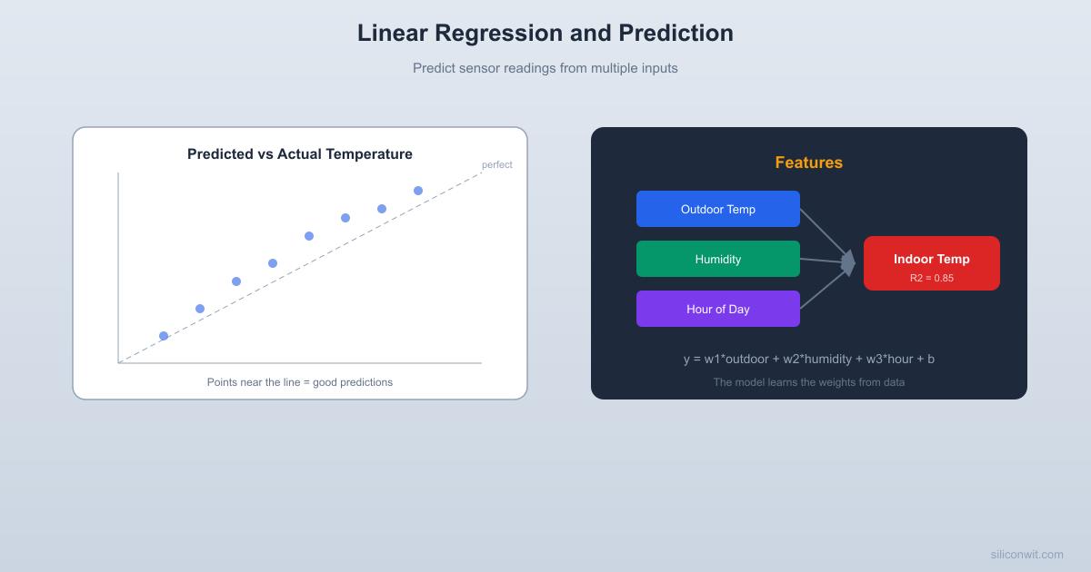
You have a set of environmental sensors measuring outdoor temperature, relative humidity, and time of day. You want to predict the indoor temperature of a building. This is a real problem in building automation, HVAC control, and energy management.

We will generate a synthetic dataset that mimics realistic sensor behavior, then build a model to predict indoor temperature from the measurements.

Step 1: Generate a Realistic Sensor Dataset

Real sensor data is messy. Our synthetic data includes the physical relationships you would expect (indoor temperature tracks outdoor temperature, varies with time of day) plus noise from sensor measurement error.

import numpy as np
import matplotlib.pyplot as plt

np.random.seed(42)

n_samples = 200

# Feature 1: Outdoor temperature (Celsius), seasonal variation
outdoor_temp = 15 + 10 * np.random.randn(n_samples) * 0.5 + 5 * np.sin(np.linspace(0, 4 * np.pi, n_samples))

# Feature 2: Relative humidity (%), correlated with temperature
humidity = 60 - 0.5 * outdoor_temp + np.random.randn(n_samples) * 5
humidity = np.clip(humidity, 20, 95)

# Feature 3: Hour of day (0 to 23)
hour = np.random.randint(0, 24, n_samples).astype(float)

# Target: Indoor temperature
# Physical model: indoor temp depends on outdoor temp, humidity has a small effect,
# and there is a daily cycle (heating during work hours)
daily_cycle = 2 * np.sin(2 * np.pi * (hour - 6) / 24)  # peaks around noon
indoor_temp = (
    0.4 * outdoor_temp          # tracks outdoor temp
    - 0.05 * humidity            # higher humidity slightly lowers indoor temp
    + daily_cycle                # HVAC daily cycle
    + 18                         # baseline indoor temp
    + np.random.randn(n_samples) * 1.0  # sensor noise
)

print(f"Dataset shape: {n_samples} samples, 3 features")
print(f"\nFeature ranges:")
print(f"  Outdoor temp: {outdoor_temp.min():.1f} to {outdoor_temp.max():.1f} C")
print(f"  Humidity:     {humidity.min():.1f} to {humidity.max():.1f} %")
print(f"  Hour:         {hour.min():.0f} to {hour.max():.0f}")
print(f"  Indoor temp:  {indoor_temp.min():.1f} to {indoor_temp.max():.1f} C (target)")

# Quick visualization
fig, axes = plt.subplots(1, 3, figsize=(14, 4))

axes[0].scatter(outdoor_temp, indoor_temp, alpha=0.5, s=15, color='steelblue')
axes[0].set_xlabel('Outdoor Temp (C)')
axes[0].set_ylabel('Indoor Temp (C)')
axes[0].set_title('Indoor vs Outdoor Temperature')

axes[1].scatter(humidity, indoor_temp, alpha=0.5, s=15, color='seagreen')
axes[1].set_xlabel('Humidity (%)')
axes[1].set_ylabel('Indoor Temp (C)')
axes[1].set_title('Indoor Temp vs Humidity')

axes[2].scatter(hour, indoor_temp, alpha=0.5, s=15, color='coral')
axes[2].set_xlabel('Hour of Day')
axes[2].set_ylabel('Indoor Temp (C)')
axes[2].set_title('Indoor Temp vs Hour')

for ax in axes:
    ax.grid(True, alpha=0.3)

plt.tight_layout()
plt.savefig('sensor_data_exploration.png', dpi=100)
plt.show()
print("\nPlot saved as sensor_data_exploration.png")

Step 2: Feature Scaling

Linear regression itself does not require feature scaling for correctness. The math works either way. But scaling matters for two practical reasons:

Coefficient interpretation. After scaling, the coefficients tell you which feature has the most influence. Without scaling, a coefficient is entangled with the feature’s units.
Numerical stability. Features with very different scales (humidity in 20 to 95 vs hour in 0 to 23) can cause numerical issues in some algorithms. Gradient descent (Lesson 5) is especially sensitive to this.

scikit-learn’s StandardScaler subtracts the mean and divides by the standard deviation, so every feature ends up with mean 0 and standard deviation 1.

import numpy as np
from sklearn.preprocessing import StandardScaler

np.random.seed(42)

# Recreate the dataset (same as above)
n_samples = 200
outdoor_temp = 15 + 10 * np.random.randn(n_samples) * 0.5 + 5 * np.sin(np.linspace(0, 4 * np.pi, n_samples))
humidity = 60 - 0.5 * outdoor_temp + np.random.randn(n_samples) * 5
humidity = np.clip(humidity, 20, 95)
hour = np.random.randint(0, 24, n_samples).astype(float)
daily_cycle = 2 * np.sin(2 * np.pi * (hour - 6) / 24)
indoor_temp = 0.4 * outdoor_temp - 0.05 * humidity + daily_cycle + 18 + np.random.randn(n_samples) * 1.0

# Stack features into a matrix
X = np.column_stack([outdoor_temp, humidity, hour])
y = indoor_temp

print("Before scaling:")
print(f"  Feature means:  {X.mean(axis=0)}")
print(f"  Feature stds:   {X.std(axis=0)}")

scaler = StandardScaler()
X_scaled = scaler.fit_transform(X)

print("\nAfter scaling:")
print(f"  Feature means:  {X_scaled.mean(axis=0).round(6)}")
print(f"  Feature stds:   {X_scaled.std(axis=0).round(6)}")

Important: Fit on Training Data Only

When you scale features, fit the scaler on the training data only. Then use the same scaler to transform the test data. If you fit on the entire dataset, information from the test set leaks into the training process. This is called data leakage and it produces overly optimistic evaluation results.

Step 3: Train/Test Split and Model Training

import numpy as np
import matplotlib.pyplot as plt
from sklearn.model_selection import train_test_split
from sklearn.preprocessing import StandardScaler
from sklearn.linear_model import LinearRegression

np.random.seed(42)

# ── Generate Dataset ──
n_samples = 200
outdoor_temp = 15 + 10 * np.random.randn(n_samples) * 0.5 + 5 * np.sin(np.linspace(0, 4 * np.pi, n_samples))
humidity = 60 - 0.5 * outdoor_temp + np.random.randn(n_samples) * 5
humidity = np.clip(humidity, 20, 95)
hour = np.random.randint(0, 24, n_samples).astype(float)
daily_cycle = 2 * np.sin(2 * np.pi * (hour - 6) / 24)
indoor_temp = 0.4 * outdoor_temp - 0.05 * humidity + daily_cycle + 18 + np.random.randn(n_samples) * 1.0

X = np.column_stack([outdoor_temp, humidity, hour])
y = indoor_temp

# ── Split ──
X_train, X_test, y_train, y_test = train_test_split(X, y, test_size=0.3, random_state=42)
print(f"Training set: {X_train.shape[0]} samples")
print(f"Test set:     {X_test.shape[0]} samples")

# ── Scale (fit on training data only) ──
scaler = StandardScaler()
X_train_scaled = scaler.fit_transform(X_train)
X_test_scaled = scaler.transform(X_test)  # use the SAME scaler, no re-fitting

# ── Train ──
model = LinearRegression()
model.fit(X_train_scaled, y_train)

# ── Coefficients ──
feature_names = ['Outdoor Temp', 'Humidity', 'Hour']
print("\nLearned coefficients (scaled features):")
for name, coef in zip(feature_names, model.coef_):
    print(f"  {name:15s}: {coef:+.4f}")
print(f"  {'Intercept':15s}: {model.intercept_:+.4f}")

# ── Predictions ──
y_train_pred = model.predict(X_train_scaled)
y_test_pred = model.predict(X_test_scaled)

print(f"\nSample predictions (first 5 test samples):")
print(f"  {'Actual':<10} {'Predicted':<10} {'Error':<10}")
for actual, predicted in zip(y_test[:5], y_test_pred[:5]):
    print(f"  {actual:<10.2f} {predicted:<10.2f} {actual - predicted:<10.2f}")

Step 4: Evaluation Metrics

Three metrics give you different views of model quality.

  Regression Evaluation Metrics
  ──────────────────────────────────────────────

  MSE (Mean Squared Error)
    = average of (actual - predicted)^2
    Penalizes large errors heavily (squaring).
    Units: squared units of the target.

  MAE (Mean Absolute Error)
    = average of |actual - predicted|
    Treats all errors equally.
    Units: same as the target.

  R-squared (Coefficient of Determination)
    = 1 - (sum of squared residuals) / (total variance)
    Ranges from 0 to 1 (can be negative for bad models).
    1.0 = perfect predictions.
    0.0 = model is no better than predicting the mean.

import numpy as np
import matplotlib.pyplot as plt
from sklearn.model_selection import train_test_split
from sklearn.preprocessing import StandardScaler
from sklearn.linear_model import LinearRegression
from sklearn.metrics import mean_squared_error, mean_absolute_error, r2_score

np.random.seed(42)

# ── Generate, split, scale, train (same pipeline) ──
n_samples = 200
outdoor_temp = 15 + 10 * np.random.randn(n_samples) * 0.5 + 5 * np.sin(np.linspace(0, 4 * np.pi, n_samples))
humidity = 60 - 0.5 * outdoor_temp + np.random.randn(n_samples) * 5
humidity = np.clip(humidity, 20, 95)
hour = np.random.randint(0, 24, n_samples).astype(float)
daily_cycle = 2 * np.sin(2 * np.pi * (hour - 6) / 24)
indoor_temp = 0.4 * outdoor_temp - 0.05 * humidity + daily_cycle + 18 + np.random.randn(n_samples) * 1.0

X = np.column_stack([outdoor_temp, humidity, hour])
y = indoor_temp

X_train, X_test, y_train, y_test = train_test_split(X, y, test_size=0.3, random_state=42)

scaler = StandardScaler()
X_train_scaled = scaler.fit_transform(X_train)
X_test_scaled = scaler.transform(X_test)

model = LinearRegression()
model.fit(X_train_scaled, y_train)

y_train_pred = model.predict(X_train_scaled)
y_test_pred = model.predict(X_test_scaled)

# ── Evaluation ──
print("=" * 45)
print("EVALUATION RESULTS")
print("=" * 45)
print(f"\n{'Metric':<20} {'Train':<12} {'Test':<12}")
print("-" * 44)
print(f"{'MSE':<20} {mean_squared_error(y_train, y_train_pred):<12.4f} {mean_squared_error(y_test, y_test_pred):<12.4f}")
print(f"{'MAE':<20} {mean_absolute_error(y_train, y_train_pred):<12.4f} {mean_absolute_error(y_test, y_test_pred):<12.4f}")
print(f"{'R-squared':<20} {r2_score(y_train, y_train_pred):<12.4f} {r2_score(y_test, y_test_pred):<12.4f}")
print(f"{'RMSE':<20} {np.sqrt(mean_squared_error(y_train, y_train_pred)):<12.4f} {np.sqrt(mean_squared_error(y_test, y_test_pred)):<12.4f}")

print(f"\nInterpretation:")
test_rmse = np.sqrt(mean_squared_error(y_test, y_test_pred))
test_r2 = r2_score(y_test, y_test_pred)
print(f"  RMSE of {test_rmse:.2f} C means predictions are off by about {test_rmse:.1f} degrees on average.")
print(f"  R-squared of {test_r2:.3f} means the model explains {test_r2 * 100:.1f}% of the variance in indoor temperature.")

# ── Plot: Predicted vs Actual ──
fig, axes = plt.subplots(1, 2, figsize=(12, 5))

# Predicted vs Actual
axes[0].scatter(y_test, y_test_pred, alpha=0.6, s=20, color='steelblue')
min_val = min(y_test.min(), y_test_pred.min())
max_val = max(y_test.max(), y_test_pred.max())
axes[0].plot([min_val, max_val], [min_val, max_val], 'r--', linewidth=2, label='Perfect prediction')
axes[0].set_xlabel('Actual Indoor Temp (C)')
axes[0].set_ylabel('Predicted Indoor Temp (C)')
axes[0].set_title(f'Predicted vs Actual (R² = {test_r2:.3f})')
axes[0].legend()
axes[0].grid(True, alpha=0.3)

# Error distribution
errors = y_test - y_test_pred
axes[1].hist(errors, bins=20, color='steelblue', edgecolor='white', alpha=0.7)
axes[1].axvline(x=0, color='red', linestyle='--', linewidth=2)
axes[1].set_xlabel('Prediction Error (C)')
axes[1].set_ylabel('Count')
axes[1].set_title(f'Error Distribution (MAE = {mean_absolute_error(y_test, y_test_pred):.2f} C)')
axes[1].grid(True, alpha=0.3)

plt.tight_layout()
plt.savefig('regression_evaluation.png', dpi=100)
plt.show()
print("\nPlot saved as regression_evaluation.png")

Step 5: Residual Analysis

Metrics tell you how wrong the model is. Residual analysis tells you why. If the errors show a pattern, the model is missing something systematic.

import numpy as np
import matplotlib.pyplot as plt
from sklearn.model_selection import train_test_split
from sklearn.preprocessing import StandardScaler
from sklearn.linear_model import LinearRegression

np.random.seed(42)

# ── Full pipeline ──
n_samples = 200
outdoor_temp = 15 + 10 * np.random.randn(n_samples) * 0.5 + 5 * np.sin(np.linspace(0, 4 * np.pi, n_samples))
humidity = 60 - 0.5 * outdoor_temp + np.random.randn(n_samples) * 5
humidity = np.clip(humidity, 20, 95)
hour = np.random.randint(0, 24, n_samples).astype(float)
daily_cycle = 2 * np.sin(2 * np.pi * (hour - 6) / 24)
indoor_temp = 0.4 * outdoor_temp - 0.05 * humidity + daily_cycle + 18 + np.random.randn(n_samples) * 1.0

X = np.column_stack([outdoor_temp, humidity, hour])
y = indoor_temp

X_train, X_test, y_train, y_test = train_test_split(X, y, test_size=0.3, random_state=42)

scaler = StandardScaler()
X_train_scaled = scaler.fit_transform(X_train)
X_test_scaled = scaler.transform(X_test)

model = LinearRegression()
model.fit(X_train_scaled, y_train)
y_test_pred = model.predict(X_test_scaled)

residuals = y_test - y_test_pred

# ── Residual Plots ──
fig, axes = plt.subplots(1, 3, figsize=(15, 4))

# Residuals vs predicted
axes[0].scatter(y_test_pred, residuals, alpha=0.5, s=20, color='steelblue')
axes[0].axhline(y=0, color='red', linestyle='--', linewidth=2)
axes[0].set_xlabel('Predicted Value')
axes[0].set_ylabel('Residual')
axes[0].set_title('Residuals vs Predicted')

# Residuals vs each feature
feature_names = ['Outdoor Temp', 'Humidity', 'Hour']
for i, (ax, name) in enumerate(zip(axes[1:], ['Outdoor Temp', 'Hour'])):
    feature_idx = [0, 2][i]  # outdoor temp and hour
    ax.scatter(X_test[:, feature_idx], residuals, alpha=0.5, s=20, color='seagreen')
    ax.axhline(y=0, color='red', linestyle='--', linewidth=2)
    ax.set_xlabel(name)
    ax.set_ylabel('Residual')
    ax.set_title(f'Residuals vs {name}')

for ax in axes:
    ax.grid(True, alpha=0.3)

plt.tight_layout()
plt.savefig('residual_analysis.png', dpi=100)
plt.show()

print("Residual analysis:")
print(f"  Mean residual:  {residuals.mean():.4f} (should be near 0)")
print(f"  Std residual:   {residuals.std():.4f}")
print(f"  Max |residual|: {np.abs(residuals).max():.4f}")
print()
print("Look at the 'Residuals vs Hour' plot.")
print("If you see a sine-wave pattern, the linear model is missing the daily cycle.")
print("A linear model cannot capture sin(hour) without feature engineering.")
print("Solution: add sin(hour) and cos(hour) as features (next section).")
print("\nPlot saved as residual_analysis.png")

Step 6: Feature Engineering Fixes the Residuals

The residual plot against hour likely shows a sinusoidal pattern. The model is linear, and the daily cycle is a sine wave. A linear model cannot capture a nonlinear relationship unless you give it the right features.

The fix: instead of using hour directly, create sin(2*pi*hour/24) and cos(2*pi*hour/24) as features. This is feature engineering, and it is often more effective than switching to a more complex model.

import numpy as np
import matplotlib.pyplot as plt
from sklearn.model_selection import train_test_split
from sklearn.preprocessing import StandardScaler
from sklearn.linear_model import LinearRegression
from sklearn.metrics import mean_squared_error, r2_score

np.random.seed(42)

# ── Generate data ──
n_samples = 200
outdoor_temp = 15 + 10 * np.random.randn(n_samples) * 0.5 + 5 * np.sin(np.linspace(0, 4 * np.pi, n_samples))
humidity = 60 - 0.5 * outdoor_temp + np.random.randn(n_samples) * 5
humidity = np.clip(humidity, 20, 95)
hour = np.random.randint(0, 24, n_samples).astype(float)
daily_cycle = 2 * np.sin(2 * np.pi * (hour - 6) / 24)
indoor_temp = 0.4 * outdoor_temp - 0.05 * humidity + daily_cycle + 18 + np.random.randn(n_samples) * 1.0

# ── Original features ──
X_original = np.column_stack([outdoor_temp, humidity, hour])

# ── Engineered features: replace hour with sin and cos ──
hour_sin = np.sin(2 * np.pi * hour / 24)
hour_cos = np.cos(2 * np.pi * hour / 24)
X_engineered = np.column_stack([outdoor_temp, humidity, hour_sin, hour_cos])

y = indoor_temp

# ── Compare both feature sets ──
results = {}
for name, X_data, feat_names in [
    ("Original (3 features)", X_original, ['OutTemp', 'Humidity', 'Hour']),
    ("Engineered (4 features)", X_engineered, ['OutTemp', 'Humidity', 'sin(hour)', 'cos(hour)']),
]:
    X_tr, X_te, y_tr, y_te = train_test_split(X_data, y, test_size=0.3, random_state=42)
    sc = StandardScaler()
    X_tr_s = sc.fit_transform(X_tr)
    X_te_s = sc.transform(X_te)

    m = LinearRegression()
    m.fit(X_tr_s, y_tr)
    y_pred = m.predict(X_te_s)

    rmse = np.sqrt(mean_squared_error(y_te, y_pred))
    r2 = r2_score(y_te, y_pred)
    results[name] = {'rmse': rmse, 'r2': r2, 'residuals': y_te - y_pred}

    print(f"\n{name}:")
    print(f"  RMSE: {rmse:.4f} C")
    print(f"  R²:   {r2:.4f}")
    print(f"  Coefficients:")
    for fn, c in zip(feat_names, m.coef_):
        print(f"    {fn:12s}: {c:+.4f}")

# ── Compare residuals ──
fig, axes = plt.subplots(1, 2, figsize=(12, 5))
X_tr, X_te, y_tr, y_te = train_test_split(X_original, y, test_size=0.3, random_state=42)

for ax, (name, data) in zip(axes, results.items()):
    ax.scatter(X_te[:, 2] if 'Original' in name else np.sin(2*np.pi*X_te[:, 2]/24),
               data['residuals'], alpha=0.5, s=20, color='steelblue')
    ax.axhline(y=0, color='red', linestyle='--', linewidth=2)
    x_label = 'Hour' if 'Original' in name else 'sin(hour)'
    ax.set_xlabel(x_label)
    ax.set_ylabel('Residual')
    ax.set_title(f'{name}\nRMSE={data["rmse"]:.3f}, R²={data["r2"]:.3f}')
    ax.grid(True, alpha=0.3)

plt.tight_layout()
plt.savefig('feature_engineering_comparison.png', dpi=100)
plt.show()

print("\nThe engineered features capture the daily cycle that raw hour cannot.")
print("Feature engineering often matters more than the choice of algorithm.")
print("\nPlot saved as feature_engineering_comparison.png")

Connect to Applied Math

Encoding cyclic variables as sine and cosine pairs is the same idea as Fourier decomposition from the Applied Mathematics course. You are projecting a periodic signal onto its fundamental frequency components. The linear model can then learn the amplitude and phase through its coefficients.

The Complete Pipeline

Here is the full pipeline in one script, from data generation to final evaluation.

  The ML Regression Pipeline
  ──────────────────────────────────────────────

  Raw Data
    │
    ├── Feature Engineering
    │     (encode cyclic variables, add derived features)
    │
    ├── Train/Test Split
    │     (70/30 or 80/20, random shuffle)
    │
    ├── Feature Scaling
    │     (fit scaler on train ONLY, transform both)
    │
    ├── Model Training
    │     (LinearRegression.fit on training data)
    │
    ├── Prediction
    │     (model.predict on test data)
    │
    ├── Evaluation
    │     (MSE, MAE, R-squared on test set)
    │
    └── Residual Analysis
          (are errors random or patterned?)
          If patterned: go back to Feature Engineering

Key Takeaways

Multiple features, same idea. Linear regression with multiple inputs is the same least-squares fitting you know, extended to higher dimensions. scikit-learn handles the linear algebra.
Scale features, fit on training data only. StandardScaler ensures all features contribute proportionally. Fitting on the full dataset is data leakage.
RMSE has the same units as your target. An RMSE of 1.5 C means your predictions are off by about 1.5 degrees on average. MSE squares the units, so interpret RMSE instead.
R-squared tells you the fraction of variance explained. An R-squared of 0.85 means the model captures 85% of the variation in the target. The remaining 15% is noise or missing features.
Residual analysis reveals what the model misses. If residuals show a pattern, the model is systematically wrong. Feature engineering (not a fancier algorithm) is usually the fix.

What is Next

In Lesson 3: Classification: Yes or No Decisions, you will move from predicting continuous values to making binary decisions. Instead of “what temperature?” the question becomes “is this sensor board defective?” The math changes only slightly, but the evaluation metrics change completely.

Comments

Loading comments...