Calculus for Engineers

Modified: Mar. 15, 2026

Published: Mar. 2, 2026

Become Contributor Expert Support

This is not a full calculus course. This is the parts of calculus that engineers reach for every single day. If calculus were a toolbox, we are going to focus on the hammer, the screwdriver, and the wrench: the tools you will actually hold in your hands, not the specialty bits that stay in the drawer. #Calculus #Engineering #AppliedMath

Derivatives: How Fast Is It Changing?

A derivative answers one question: at this exact moment, how fast is something changing?

You are driving. Your odometer reads distance. Your speedometer reads the derivative of distance with respect to time. Your speed tells you how fast the distance is accumulating right now.

Your car’s speedometer is literally displaying the derivative of your odometer reading. Every time you glance at the speedometer, you are reading a derivative.

That is the entire concept. The derivative of position is velocity. The derivative of velocity is acceleration. The derivative of charge is current. The derivative of temperature with respect to position is the temperature gradient. Every time you ask “how fast is this quantity changing?” you are asking for a derivative.

The Derivative as a Slope

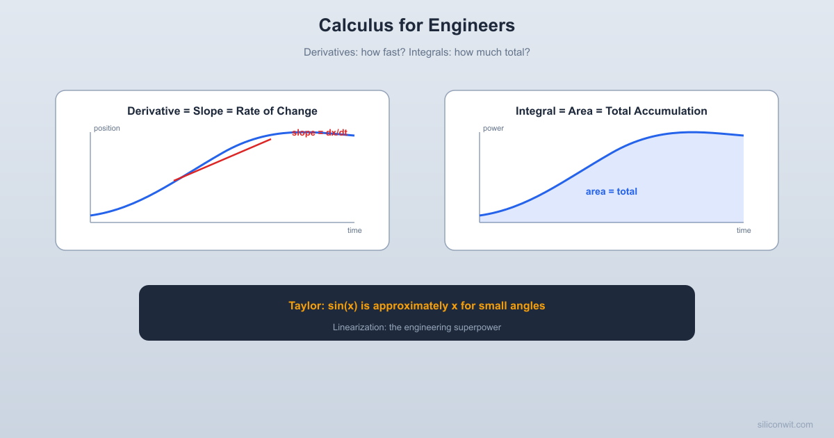
Graphically, the derivative at a point is the slope of the tangent line at that point. If you plot temperature versus time for a cooling cup of coffee, the derivative at any moment tells you how fast the coffee is cooling right then.

  T (C)
  90 |*
     |  *
     |    *
     |      *  <-- steep slope here = fast cooling
     |         *
     |            *
     |               *   *   <-- gentle slope = slow cooling
     |                       *   *   *   *
  22 |--------------------------------------- T_room
     +---------------------------------------- t (min)
     0    5    10   15   20   25   30   35

When the curve is steep, the derivative is large (the coffee is cooling quickly). When the curve flattens out, the derivative approaches zero (the coffee has nearly reached room temperature).

Key Derivatives Engineers Use

Here are the derivatives that appear most often in engineering work:

The exponential function is special: its derivative is proportional to itself. That is why it appears in every system involving growth or decay, from RC circuits to population dynamics to radioactive decay.

Worked Example: Current from Charge

If the charge on a capacitor varies as , the current flowing is:

The negative sign tells you the charge is decreasing (the capacitor is discharging). The current magnitude starts at and decays exponentially. This is the discharge curve you see in every electronics textbook, and it comes directly from taking a derivative.

Integrals: How Much Has Accumulated?

If derivatives answer “how fast?”, integrals answer “how much in total?” Your monthly electricity bill is the integral of your power usage over time: the utility company measures how many watts you draw each moment, accumulates that over the billing period, and charges you for the total kilowatt-hours.

You are driving at a varying speed. Your speedometer changes moment to moment. How far did you travel in total? You add up all the tiny distances: speed times a tiny time interval, over and over. In the limit, that sum becomes an integral:

Graphically, the integral is the area under the curve. The area under a velocity-time graph is the total distance traveled.

  v (m/s)
  20 |        ****
     |      **    **
     |    **        **
  10 |  **            **
     | *                **
     |*                   ****
   0 +----------------------------- t (s)
     0    2    4    6    8    10

     The shaded area = total distance traveled

Key Integrals Engineers Use

Worked Example: Energy from Power

A solar panel produces power that varies throughout the day. The total energy harvested is:

If the power follows a rough sinusoidal pattern (zero at dawn and dusk, peak at noon):

where is the length of daylight. The total energy is:

For and :

That is a useful estimate for sizing a battery bank.

The Fundamental Theorem of Calculus

The fundamental theorem of calculus says that differentiation and integration are inverse operations. If you integrate a function and then differentiate the result, you get back the original function:

This is not just a mathematical curiosity. It means that if you know the rate of change of something (the derivative), you can find the total change by integrating. And if you know the total accumulated quantity, you can find the rate by differentiating. Velocity and position. Current and charge. Power and energy. These pairs are connected by the fundamental theorem.

Taylor Series: Approximation is a Superpower

Here is one of the most useful ideas in all of applied mathematics: any smooth function can be approximated near a point by a polynomial. The Taylor series of a function around the point is:

Why Engineers Love This

Most of the time, you only need the first one or two terms. That turns a complicated function into a simple linear or quadratic approximation.

The small-angle approximation:

For small (in radians):

This is the first-term Taylor expansion around . It turns the nonlinear pendulum equation into a linear one, which you can solve exactly. For rad (about 17 degrees), the error in is less than 1.5%.

The exponential approximation:

This appears constantly in engineering. For a small perturbation around an operating point, turns exponential behavior into linear behavior. This is the foundation of small-signal analysis in electronics.

Linearization:

The Taylor series with just the first two terms is linearization. You are replacing a curved function with a straight line that touches the curve at one point. This is how engineers turn nonlinear problems into linear ones, which are far easier to solve.

How Good Is the Approximation?

import numpy as np

theta = np.array([0.1, 0.2, 0.3, 0.5, 1.0])
sin_exact = np.sin(theta)
sin_approx = theta

print("theta (rad) | sin(theta) | approx  | error (%)")
print("-" * 50)
for i in range(len(theta)):
    error = abs(sin_exact[i] - sin_approx[i]) / sin_exact[i] * 100
    print(f"  {theta[i]:.1f}       |  {sin_exact[i]:.5f}  | {sin_approx[i]:.5f} | {error:.2f}%")

Output:

theta (rad) | sin(theta) | approx  | error (%)
--------------------------------------------------
  0.1       |  0.09983  | 0.10000 | 0.17%
  0.2       |  0.19867  | 0.20000 | 0.67%
  0.3       |  0.29552  | 0.30000 | 1.52%
  0.5       |  0.47943  | 0.50000 | 4.29%
  1.0       |  0.84147  | 1.00000 | 18.83%

At 0.3 radians the approximation is excellent. At 1.0 radian it is poor. Knowing the domain of validity of your approximations is critical.

The Chain Rule: Compound Rates of Change

The chain rule tells you how to differentiate a composition of functions. If , then:

In plain language: if depends on , and depends on , then the rate of change of with respect to is the product of the two intermediate rates.

Engineering Application: Sensor Calibration

A thermistor’s resistance varies with temperature:

An ADC converts this resistance to a digital reading through a voltage divider. The voltage across the thermistor is:

If you want to know how the voltage reading changes with temperature, you need the chain rule:

Each piece is straightforward on its own. The chain rule lets you compose them. This tells you the sensitivity of your measurement system: how many millivolts per degree of temperature change.

Engineering Application: Unit Conversion in Rates

The chain rule is also why unit conversions work the way they do for rates. If a car travels at 90 km/h and you want m/s:

Each conversion factor is a in a chain of variable substitutions.

Numerical Differentiation and Integration

In practice, you often have discrete data, not continuous functions. A sensor gives you temperature readings every second, not a formula. You need numerical methods.

Numerical Derivative: Finite Differences

The simplest approximation to a derivative uses two adjacent data points:

This is the central difference formula. It is more accurate than the forward difference because it uses information from both sides of the point.

Numerical Integral: The Trapezoidal Rule

To integrate discrete data, approximate the area under the curve as a series of trapezoids:

Python: Differentiation and Integration of Sensor Data

import numpy as np

# Simulated sensor data: temperature readings every 1 second
t = np.arange(0, 60, 1.0)          # time in seconds
T = 90 * np.exp(-0.05 * t) + 22    # cooling curve (C)

# Numerical derivative: rate of cooling (C/s)
dT_dt = np.gradient(T, t)

# Numerical integral: total "degree-seconds" of cooling
# (useful for thermal energy calculations)
total = np.trapz(T - 22, t)

print(f"Initial cooling rate: {dT_dt[0]:.2f} C/s")
print(f"Cooling rate at t=30s: {dT_dt[30]:.2f} C/s")
print(f"Integrated thermal energy (proportional): {total:.1f} degree-seconds")

NumPy’s np.gradient() computes the central difference, and np.trapz() computes the trapezoidal integral. These two functions handle 90% of the numerical calculus you will ever need.

Putting It All Together

Calculus gives you four essential tools:

These are not separate topics. They are facets of one idea: calculus is the mathematics of change and accumulation. Every engineering system changes over time, and calculus is how you describe, predict, and control that change.

In the next lesson, we will see how linear algebra provides the other essential framework: the mathematics of systems, where multiple quantities interact simultaneously.