Uncertainty and the Limits of Knowledge

Modified: Mar. 15, 2026

Published: Mar. 6, 2026

Become Contributor Expert Support

Engineering is built on measurement, calculation, and prediction. But none of these are perfect. Every sensor has noise, every model has assumptions, and every forecast has a horizon beyond which it becomes guesswork. Understanding the limits of knowledge is not a reason for despair; it is the foundation of responsible design. Engineers who know what they cannot know build systems that survive the unexpected. #Uncertainty #EngineeringDesign #ComplexSystems

Every Number Has Error Bars

When you measure the length of a steel beam with a tape measure, you might record 2.450 meters. But the true length is not exactly 2.450 meters. It might be 2.4497 or 2.4503. The tape measure has a resolution limit, your reading angle introduces parallax, and the beam itself expands and contracts with temperature.

Sources of Measurement Error

Propagation of Uncertainty

Uncertainty compounds through calculations. If you multiply two measured quantities, each with 1% uncertainty, the result has roughly 1.4% uncertainty (the uncertainties add in quadrature). For a system with dozens of measured inputs feeding into a design calculation, the final uncertainty can be surprisingly large.

Consider a simple stress calculation: . If the force is known to and the cross-sectional area is known to , the stress is uncertain by roughly . That 3.6% might be the difference between a safe design and a marginal one.

This is why safety factors exist. They are not there because engineers are bad at math. They are there because engineers are honest about their math.

A Real-World Example: The Mars Climate Orbiter

In 1999, NASA’s Mars Climate Orbiter was lost because one engineering team used imperial units (pound-force seconds) while another used metric units (newton-seconds) for thruster impulse calculations. The error was not in the physics or the instruments. It was in the interface between two groups, each of which had internally consistent and accurate data.

The total cost of the mission was approximately 327.6 million USD. The root cause was not a measurement error but a failure to explicitly document and verify units at the system boundary. This is a case where uncertainty was not the problem; unexamined assumptions were.

Statistical Thinking in Engineering

Engineers who work with uncertainty need at least a basic statistical vocabulary:

The temptation is to take the average and discard the spread. Resist this temptation. The spread is information. A measurement with a mean of 5.0 V and a standard deviation of 0.01 V tells a very different story from one with the same mean and a standard deviation of 0.5 V.

Chaos: Deterministic but Unpredictable

In the early 1960s, meteorologist Edward Lorenz was running a simple weather simulation on a computer. To save time, he restarted a run from the middle, entering the intermediate values by hand. But he rounded one number from 0.506127 to 0.506. The result was a completely different weather pattern.

This was not a bug. It was chaos theory in action.

The Butterfly Effect in Engineering

Lorenz’s discovery has real consequences for engineers:

Weather and climate: You can predict tomorrow’s weather reasonably well, next week’s weather poorly, and next month’s weather hardly at all. This is not because meteorologists are incompetent. It is because the atmosphere is a chaotic system with a prediction horizon of roughly 10 to 14 days.

Turbulent flow: The Navier-Stokes equations governing fluid dynamics are deterministic. But turbulent flow is chaotic. Two nearly identical initial flow states diverge exponentially. This is why you cannot predict exactly where a plume of smoke will go, even though the physics is completely known.

Electronic oscillators: Certain nonlinear circuits exhibit chaotic behavior. A Chua’s circuit, for example, follows deterministic equations but produces an output that looks random. The same sensitivity to initial conditions applies.

The Practical Consequence

For engineers, chaos means that some systems cannot be predicted beyond a certain time horizon, no matter how good your instruments or how powerful your computer. The response is not to give up on prediction. It is to understand the prediction horizon and design accordingly.

Weather forecasters use ensemble methods: run the simulation hundreds of times with slightly different initial conditions and look at the spread of outcomes. If all ensemble members agree, confidence is high. If they diverge, you know the forecast is unreliable.

Engineers can apply the same principle to any system with chaotic behavior.

Lyapunov Time: The Prediction Horizon

For any chaotic system, there is a characteristic timescale called the Lyapunov time, beyond which prediction becomes unreliable. This timescale depends on the system:

The Lyapunov time tells you how far ahead your model can reliably predict. For engineering purposes, this determines whether prediction-based control is feasible (if the Lyapunov time is long relative to your control cycle) or whether you need reactive, feedback-based strategies (if the Lyapunov time is short).

A control system for a turbulent combustion process cannot predict the flow pattern 10 seconds ahead. But it can measure the current state and adjust in real time. The uncertainty does not make control impossible. It changes the kind of control that works.

Complexity and Emergence

Chaos involves simple systems with sensitive dependence on initial conditions. Complexity involves systems with many interacting parts that produce collective behavior no individual part exhibits.

Emergent Behavior

Consider traffic flow. Each driver follows simple rules: maintain speed, keep distance, brake when needed. No driver intends to create a traffic jam. But jams emerge from the interaction of thousands of drivers making independent decisions. The jam is an emergent property of the system, not a feature of any individual car.

Other examples of emergence:

Why Emergence Matters for Engineers

When you design a component, you can test it in isolation. But the behavior of the system containing that component may surprise you. A software module that passes all unit tests can cause a system failure when it interacts with other modules under load. A structural member that meets all specifications can contribute to a resonance failure when combined with other members.

The lesson: testing components is necessary but not sufficient. You must also test the system, and you must accept that some system-level behaviors will only appear in the field.

Tightly Coupled Systems

Sociologist Charles Perrow introduced the concept of “normal accidents” in his study of complex systems. He argued that in tightly coupled systems (where components interact quickly and with little slack), failures can cascade faster than operators can respond.

A power grid is tightly coupled: a failure at one node can cascade through the network in seconds. The Northeast blackout of 2003 started with an alarm system failure at a utility in Ohio, combined with untrimmed trees touching power lines. Within hours, 55 million people lost power across the northeastern United States and Ontario, Canada.

For engineers designing tightly coupled systems, the implication is clear: you must design for cascading failure, not just individual component failure. Circuit breakers, rate limiters, bulkheads, and graceful degradation mechanisms are all strategies for preventing local failures from becoming system-wide catastrophes.

Known Unknowns and Unknown Unknowns

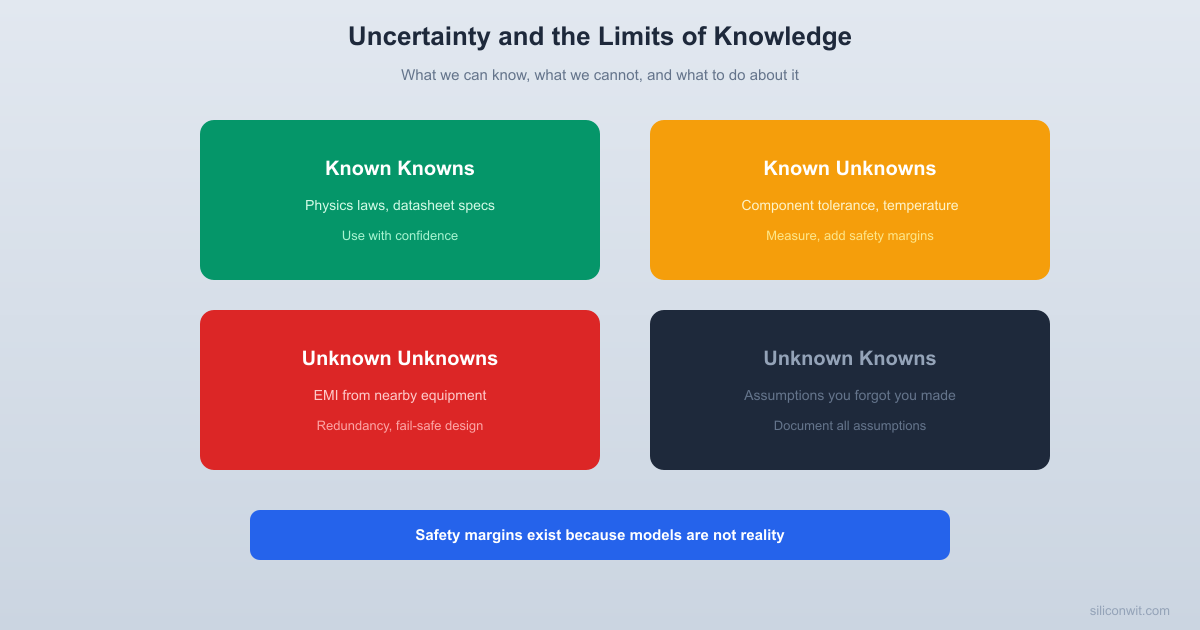
In 2002, U.S. Secretary of Defense Donald Rumsfeld gave a press conference that was widely mocked but contained a genuinely useful epistemological framework:

“There are known knowns: things we know we know. There are known unknowns: things we know we don’t know. But there are also unknown unknowns: things we don’t know we don’t know.”

Engineers deal with all three categories constantly.

  The Known/Unknown Matrix

           |  Known to us   | Unknown to us
  ---------+----------------+------------------
  Known    | KNOWN KNOWNS   | KNOWN UNKNOWNS
  to exist | Steel strength | Wind load in a
           | at 20 C        | 100-year storm
           | Ohm's law      | Exact user count
  ---------+----------------+------------------
  Unknown  | (impossible    | UNKNOWN UNKNOWNS
  to exist | by definition) | Aeroelastic flutter
           |                | (Tacoma Narrows)
           |                | Fukushima tsunami
  ---------+----------------+------------------
    Response: Use directly    Add safety factors
              in design       Build redundancy
                              Monitor for anomalies

The Most Dangerous Category

Known unknowns are manageable. You know the soil composition at a construction site is uncertain, so you do geotechnical surveys and add safety margins. You know the exact user load on your server is unpredictable, so you build in auto-scaling.

Unknown unknowns are the dangerous ones. The Tacoma Narrows Bridge collapsed in 1940 due to aeroelastic flutter, a failure mode that bridge engineers had not considered. The Fukushima Daiichi nuclear disaster in 2011 resulted partly from a tsunami exceeding the design basis that planners had considered sufficient.

You cannot prepare for every unknown unknown. But you can build systems that degrade gracefully rather than catastrophically, and you can create feedback loops that detect anomalies before they become failures.

Converting Unknown Unknowns to Known Unknowns

The most effective strategy for handling unknown unknowns is to convert them into known unknowns as quickly as possible. This requires:

Diverse teams. People with different backgrounds, disciplines, and experiences see different risks. A mechanical engineer and a software engineer looking at the same system will identify different potential failure modes. An engineer from a different cultural context may question assumptions that the rest of the team takes for granted.

Pre-mortem analysis. Before a project launches, ask the team: “Imagine this project has failed spectacularly. What went wrong?” This technique, borrowed from cognitive psychology, activates different thinking patterns than asking “what could go wrong?” People are better at explaining a failure after it happens (even hypothetically) than at predicting it beforehand.

Incident review from other industries. Many engineering failures have analogs in other industries. A software team can learn from aviation incidents. A civil engineer can learn from software failures. The NASA Lessons Learned database and the Chemical Safety Board’s investigation reports are freely available and contain decades of hard-won knowledge.

Operational monitoring. Systems in the field generate data about how they actually behave, as opposed to how you designed them to behave. Monitoring for anomalies (unexpected patterns, out-of-range values, unusual sequences) can reveal unknown unknowns before they cause failures.

The Limits of Simulation

Modern engineering relies heavily on simulation. Finite element analysis, computational fluid dynamics, circuit simulation, and system-level modeling are all essential tools. But every simulation is a model, and every model is a simplification of reality.

What Simulations Leave Out

You can model a bridge under static load with high accuracy. But consider what a real bridge experiences that your simulation might miss:

1. Wind gusts that change direction and intensity unpredictably
2. Thermal cycling that causes daily expansion and contraction over decades
3. Corrosion that slowly reduces cross-sectional area in ways that depend on local chemistry
4. Fatigue from millions of load cycles with varying amplitude
5. Foundation settlement as soil properties change with moisture over years
6. Unexpected loads like a truck driver who ignores the weight limit sign
7. Maintenance failures when inspection schedules are cut to save budget

A simulation that accounts for items 1 through 4 might be quite good. But items 5 through 7 involve human behavior and organizational decisions that no physical simulation captures.

Verification and Validation

The simulation community distinguishes between two questions:

Verification: Does the code solve the equations correctly? This is a math question. You can answer it by comparing against analytical solutions or by running convergence studies.

Validation: Do the equations describe the real world correctly? This is a physics question. You can only answer it by comparing against experimental data.

A simulation can be perfectly verified (it solves the equations right) and still be invalid (the equations do not capture the relevant physics). Engineers must always ask both questions.

The Danger of Black Box Tools

Modern simulation tools are powerful and easy to use. A junior engineer can run a finite element analysis in an afternoon with minimal training. This is both a gift and a danger.

The gift is accessibility: more engineers can use simulation to inform their designs. The danger is that the tool can produce a plausible-looking result even when the model is fundamentally wrong. Incorrect boundary conditions, inappropriate element types, unconverged meshes, and invalid material models can all produce numbers that look reasonable but are meaningless.

The defense against this is validation: always compare simulation results against experimental data, analytical solutions, or engineering judgment. If a simulation predicts a stress concentration of 50 MPa but a handbook formula predicts 200 MPa, something is wrong with one of them. Investigate before trusting either.

Heisenberg for Engineers

The Heisenberg uncertainty principle in quantum mechanics states that you cannot simultaneously know a particle’s position and momentum with arbitrary precision. This is a fundamental limit, not a technology problem.

Engineers face an analogous challenge at the macroscopic scale: the act of measuring a system often changes the system.

Probe Effects in Electronics

When you connect an oscilloscope probe to a circuit, you add capacitance (typically 10 to 15 pF) and a parallel resistance (typically 10 megaohms). For a low-frequency, low-impedance circuit, this does not matter. For a high-frequency, high-impedance circuit, the probe changes the signal you are trying to measure.

An engineer debugging a 100 MHz signal with a 15 pF probe load might see a waveform that does not exist in the unloaded circuit. The measurement is not wrong in the sense of being inaccurate; it is wrong in the sense of measuring a different system than the one you care about.

Observer Effects in Software

Performance profiling in software has the same character. Adding instrumentation to measure execution time changes execution time. Logging I/O operations to diagnose a performance issue may itself cause I/O contention. Running a debugger changes memory layout, timing, and sometimes program behavior.

The Hawthorne Effect and Beyond

The principle extends further. In sociology and economics, measuring human behavior changes human behavior (the Hawthorne effect). Workers at the Hawthorne Works factory in the 1920s and 1930s improved their productivity simply because they knew they were being observed. The specific changes to lighting and break schedules mattered less than the attention itself.

In product testing, the test environment differs from the deployment environment in ways that matter. A device tested in a clean laboratory performs differently in a dusty factory. Software tested on a developer’s machine behaves differently on a customer’s aging hardware with background processes consuming resources. A structural prototype tested under controlled loading may respond differently to the irregular, dynamic loads of actual use.

Real Engineering Consequences of Observer Effects

The Engineering Response

The response is not to stop measuring. It is to understand how your measurement affects the system and to account for that effect. Use low-capacitance probes. Use statistical profiling instead of instrumented profiling. Run tests in environments that match production as closely as possible.

And when you cannot eliminate the observer effect, document it. “This measurement was taken with a 10x probe adding approximately 12 pF to the node” is far more useful than a bare number.

Designing for Uncertainty

Once you accept that knowledge is always incomplete, the question becomes: how do you design systems that work despite what you do not know?

Safety Margins

The simplest response to uncertainty is to add margin. If the calculated maximum stress is 200 MPa and the material’s yield strength is 300 MPa, you have a safety factor of 1.5. That margin absorbs the uncertainty in your stress calculation, the uncertainty in the material properties, and some of the unknown unknowns.

Different fields use different safety factors because they face different uncertainties:

Redundancy

Safety margins protect against larger-than-expected loads. Redundancy protects against component failure. A dual-engine aircraft can fly on one engine. A RAID array survives a disk failure. A triple-redundant flight computer tolerates a single computer malfunction.

The key insight is that redundancy only works if the failure modes are independent. Two engines mounted side by side are not truly redundant if a single fire can destroy both. Two software modules running the same algorithm are not redundant against a software bug.

Fail-Safe Design

The choice between these strategies depends on the application. A chemical plant valve should fail closed (fail-safe) to prevent a release. A fire exit should fail open (different kind of fail-safe) to allow evacuation. An aircraft flight control system must fail operational because “fail-safe” is not an option when you are at 35,000 feet.

Defense in Depth

No single strategy handles all sources of uncertainty. The most robust designs layer multiple strategies:

1. Safety margin absorbs the expected range of uncertainty in loads and material properties
2. Redundancy handles component failure within the safety margin
3. Monitoring detects when actual conditions approach or exceed the design envelope
4. Fail-safe mechanisms activate when monitoring detects a critical condition
5. Maintenance schedules address degradation before it compromises any of the above layers

Each layer protects against a different category of uncertainty. Safety margins handle known unknowns. Redundancy handles component-level failures. Monitoring detects conditions drifting outside expectations. Fail-safe mechanisms handle the cases where everything else fails. And maintenance prevents slow degradation from eroding the other layers over time.

This layered approach is called “defense in depth,” and it is used in nuclear engineering, aviation, cybersecurity, and any domain where failure has severe consequences. No single layer is perfect. But the probability of all layers failing simultaneously is much lower than the probability of any single layer failing alone.

”How Confident Should I Be?” as a Design Question

Every engineering decision carries implicit assumptions about confidence. When you select a bolt, you are confident that the manufacturer’s specification is accurate. When you choose a network protocol, you are confident that the error-correction scheme catches the error rates you will encounter.

These confidence assumptions should be explicit, not implicit.

A Practical Framework

1. List your assumptions. What facts are you relying on? Where did they come from?
2. Rate each assumption. How confident are you? Is this based on a textbook value, a manufacturer’s datasheet, a single test, or an educated guess?
3. Identify the critical ones. Which assumptions, if wrong, would cause the design to fail?
4. Address the critical, low-confidence ones. Can you test them? Can you add margin? Can you design the system so that this assumption does not matter?
5. Document everything. Future engineers (including your future self) need to know what you assumed and why.

The Confidence Spectrum

Not all knowledge deserves equal trust:

The further down this table you go, the more margin you should add.

Practical Takeaways

Exercises

1. Pick a measurement you have made recently (voltage, temperature, weight, anything). Estimate the uncertainty from at least three different sources (instrument resolution, environmental factors, measurement technique). Calculate the combined uncertainty.

2. Research the Tacoma Narrows Bridge collapse. What was the unknown unknown? How would modern engineering practice (wind tunnel testing, aeroelastic analysis) have caught it? What unknown unknowns might modern bridge engineers still be missing?

3. Find a simulation result you have used or produced. List three things the simulation assumes that reality does not guarantee. For each, estimate how much the result would change if the assumption were wrong.

4. Choose a product you use daily (phone, car, elevator, building). Identify at least two safety margins, two redundancies, and one fail-safe mechanism in its design. For each, explain what uncertainty it is designed to absorb.

Summary

Knowledge has limits, and engineering lives at those limits every day. Measurement uncertainty means no number is exact. Chaos means some systems are inherently unpredictable beyond a time horizon. Complexity means system behavior can surprise you even when you understand every component. And unknown unknowns mean you must prepare for scenarios you have not imagined. The engineering response is not to despair but to design honestly: report uncertainty, add appropriate margins, build in redundancy, test at the system level, and document your assumptions. The question “how confident should I be?” is not a philosophical curiosity. It is one of the most practical questions an engineer can ask.