Lesson 4: Velocity Kinematics and the Jacobian

Modified: Mar. 10, 2026

Published: Mar. 10, 2026

When a collaborative robot hands you a cup of coffee, it needs to move its end-effector smoothly through space at a controlled velocity. But the robot’s motors operate in joint space, spinning individual joints at angular rates. The Jacobian matrix is the bridge between these two worlds, translating joint velocities into end-effector velocities and vice versa. It also reveals dangerous configurations where the robot loses the ability to move in certain directions, and it provides the mathematical foundation for force control in human-robot collaboration. #robotics #jacobian #velocity-kinematics

🎯 Learning Objectives

By the end of this lesson, you will be able to:

Derive the Jacobian matrix for serial robot manipulators Core Theory
Compute forward and inverse velocity mappings between joint space and task space Analysis
Detect singularities and interpret their physical meaning Critical
Visualize manipulability ellipsoids using singular value decomposition Advanced
Apply the pseudoinverse method for redundant manipulators Practical
Map end-effector forces to joint torques using the Jacobian transpose Force Control

🔧 Real-World Engineering Challenge: Collaborative Robot with Force-Limited Operation

A collaborative robot on a manufacturing line must hand components to a human worker. Safety regulations (ISO/TS 15066) require that contact forces never exceed 150 N at the end-effector. The robot controller needs to continuously monitor how joint torques translate into end-effector forces, and it must detect configurations where the robot could inadvertently generate excessive forces due to mechanical advantage near singularities. The Jacobian matrix provides exactly this capability: it maps between joint-space quantities (velocities, torques) and task-space quantities (end-effector velocities, forces) in real time.

System Challenge: Safe Velocity and Force Control

Critical Engineering Questions:

Why the Jacobian Is Essential for Collaborative Robots

In traditional industrial robots behind safety cages, singularity avoidance and force control are important but not safety-critical in the same way. Collaborative robots operate in shared workspaces with humans, so the consequences of uncontrolled motion or unexpected forces are immediate and potentially dangerous. The Jacobian provides the mathematical framework for: (1) real-time velocity monitoring to ensure smooth, predictable motion, (2) force limiting by mapping joint torques to end-effector forces, (3) singularity detection to prevent loss of control, and (4) manipulability analysis to plan paths through high-dexterity configurations.

Collaborative Robot Design Challenge

Design Goal: Implement Jacobian-based velocity and force control for a collaborative 2R planar robot, with extensions to redundant 3R configurations.

Key Requirements:

Velocity Mapping: Compute end-effector velocity from joint rates in real time
Trajectory Tracking: Generate joint velocities for straight-line end-effector paths
Singularity Monitoring: Detect and avoid configurations where control degrades
Force Safety: Ensure end-effector forces stay within ISO/TS 15066 limits

📚 Fundamental Theory

What is the Jacobian?

The Jacobian is a matrix of partial derivatives that describes how small changes in one set of variables produce changes in another set. In robotics, the Jacobian relates joint velocities to end-effector velocities. Think of it as a “gear ratio matrix” that changes with the robot’s configuration.

Simple Analogies:

Bicycle Gear Ratio

On a bicycle, the gear ratio determines how pedal rotation speed translates to wheel rotation speed. The Jacobian is the robotic equivalent, but instead of a single ratio, it is an entire matrix because the robot has multiple joints and the end-effector moves in multiple directions. And unlike a fixed gear ratio, the Jacobian changes as the robot moves.

Puppet Strings

A puppeteer pulls strings (joint velocities) to make a puppet’s hand move (end-effector velocity). The relationship between string pulls and hand motion depends on the puppet’s current pose. Some poses make the hand easy to move in all directions; others make certain directions difficult or impossible. The Jacobian captures exactly this configuration-dependent relationship.

Mathematical Definition

For a general -DOF robot with forward kinematics , where is the joint variable vector and is the task-space vector, the Jacobian matrix is defined as:

The velocity relationship is then:

where is the vector of joint velocities and is the end-effector velocity vector.

Full Derivation: 2-Link Planar Robot (2R)

Let us derive the Jacobian step by step for a 2R planar robot with link lengths and , and joint angles and .

Step 1: Forward Kinematics Equations

The end-effector position in terms of the joint angles is:

Here, is measured from the positive -axis, and is the relative angle of link 2 with respect to link 1.

Step 2: Compute Partial Derivatives

We need four partial derivatives to build the Jacobian.

Partial derivatives of :

Detailed differentiation walkthrough

Consider . Differentiating with respect to : the first term gives by the chain rule. The second term gives because appears inside . Now differentiating with respect to : the first term has no dependence, so it vanishes. The second term gives . The same logic applies to the equations using derivatives of .

Step 3: Assemble the Jacobian Matrix

Combining all four partial derivatives into matrix form:

For notational convenience, let , , , :

The velocity mapping equation becomes:

Problem: Given joint velocities and , find end-effector velocity .

Method: Direct matrix multiplication.

This is always straightforward because the Jacobian is computed from the current configuration and the multiplication is a simple linear operation.

When to use: Monitoring the actual end-effector velocity from measured joint encoder rates. This is critical for collaborative robots to verify that the end-effector is not moving too fast near a human worker.

Numerical Example

Let us work through a complete numerical example to solidify the concepts. Consider a 2R robot with m, m, at configuration , . The joints are moving at rad/s and rad/s.

Compute trigonometric values:

, so ,

, so ,
Build the Jacobian:
Forward velocity mapping:

The end-effector speed is m/s.
Compute the determinant:

Since , the robot is not at a singularity and the inverse velocity mapping is well-defined.
Inverse velocity example: Suppose we want m/s, m/s (pure horizontal motion). Then:

Singularity Analysis

Singularities are configurations where the Jacobian loses rank, meaning the robot cannot generate end-effector velocities in certain directions regardless of how fast the joints move. Detecting and avoiding singularities is essential for safe robot operation.

Determinant of the Jacobian

For the 2R robot, the determinant is:

Expanding and simplifying using the identity :

Step-by-step determinant simplification

Starting from the expanded determinant:

The terms cancel:

Now apply the subtraction formula:

With and :

Therefore:

Singular Configurations

The singularity condition occurs when , which means or .

Fully Extended (theta2 = 0)
Fully Folded (theta2 = 180)

Configuration: Both links are collinear, pointing in the same direction.

Physical meaning: The end-effector is at the maximum reach . At this boundary, the robot cannot move radially outward because it is already fully stretched. Both joints can only produce tangential (circular) motion. One degree of freedom in task space is lost.

Consequence for collaborative robots: Near full extension, even small radial velocity demands require extremely large joint velocities, which is dangerous. The controller must slow down or redirect the trajectory well before reaching this configuration.

Manipulability Ellipsoids

The manipulability ellipsoid provides a geometric visualization of the robot’s velocity capability at any configuration. If all joints move at unit speed (), the set of achievable end-effector velocities forms an ellipsoid in task space. The shape and size of this ellipsoid reveal directional preferences and overall dexterity.

The ellipsoid is determined by the singular value decomposition (SVD) of the Jacobian:

where contains the singular values, defines the principal directions in task space, and defines the principal directions in joint space.

Key properties:

The semi-axes of the ellipsoid have lengths equal to the singular values
The directions of the semi-axes are the columns of
The manipulability index is (for square Jacobians)
The condition number measures isotropy ( is perfectly isotropic)

Interpreting the Manipulability Ellipsoid

Large, circular ellipsoid: The robot can move the end-effector equally well in all directions. This is the ideal configuration for collaborative tasks.

Elongated ellipsoid: The robot moves easily along the major axis but poorly along the minor axis. The task should be oriented along the major axis if possible.

Degenerate (flat) ellipsoid: One singular value is near zero, indicating proximity to a singularity. The robot effectively loses one DOF. Avoid this configuration.

Pseudoinverse for Redundant Robots

When a robot has more joints than task-space dimensions (e.g., a 3R planar robot controlling 2D position), the system is redundant. There are infinitely many joint velocity solutions for any desired end-effector velocity. The Moore-Penrose pseudoinverse provides the minimum-norm solution, and the null space allows additional objectives like singularity avoidance or joint limit avoidance.

For a redundant robot with Jacobian (), the pseudoinverse is:

The general solution to is:

where is an arbitrary vector, and projects it onto the null space of .

3-Link Planar Robot Example:

For a 3R robot with link lengths and joint angles :

The Jacobian is :

where and .

The null space has dimension , meaning one DOF of internal motion can reconfigure the arm without moving the end-effector. This extra freedom is used for:

Singularity avoidance: Choose to maximize
Joint limit avoidance: Choose to push joints away from their limits
Obstacle avoidance: Choose to move the elbow away from obstacles

Force and Torque Mapping

The Jacobian also relates end-effector forces to joint torques through the principle of virtual work. If the end-effector exerts a force on the environment, the required joint torques are given by the Jacobian transpose.

This relationship is the dual of the velocity mapping. While velocity maps forward through , force maps backward through .

Force Mapping for Collaborative Safety

ISO/TS 15066 Compliance:

Given a maximum allowable end-effector force N, the controller must ensure:

Or equivalently, limit joint torques such that the resulting end-effector force stays safe. Near singularities, small joint torques can produce large end-effector forces along certain directions, making force monitoring especially critical.

Python Code: Jacobian Computation and Velocity Mapping

import numpy as np

def jacobian_2r(theta1, theta2, L1, L2):
    """
    Compute the Jacobian matrix for a 2R planar robot.

    Parameters:
        theta1, theta2 : joint angles in radians
        L1, L2         : link lengths in meters

    Returns:
        J : 2x2 Jacobian matrix
    """
    s1 = np.sin(theta1)
    c1 = np.cos(theta1)
    s12 = np.sin(theta1 + theta2)
    c12 = np.cos(theta1 + theta2)

    J = np.array([
        [-L1*s1 - L2*s12,  -L2*s12],
        [ L1*c1 + L2*c12,   L2*c12]
    ])
    return J

def forward_velocity(J, dq):
    """
    Forward velocity mapping: joint velocities -> end-effector velocity.

    Parameters:
        J  : Jacobian matrix (m x n)
        dq : joint velocity vector (n,)

    Returns:
        dx : end-effector velocity vector (m,)
    """
    return J @ dq

def inverse_velocity(J, dx):
    """
    Inverse velocity mapping: end-effector velocity -> joint velocities.
    Uses direct inverse for square Jacobian, pseudoinverse otherwise.

    Parameters:
        J  : Jacobian matrix (m x n)
        dx : desired end-effector velocity (m,)

    Returns:
        dq : required joint velocities (n,)
    """
    if J.shape[0] == J.shape[1]:
        # Square Jacobian: use direct inverse
        det_J = np.linalg.det(J)
        if abs(det_J) < 1e-6:
            print(f"WARNING: Near singularity! det(J) = {det_J:.6f}")
            # Use damped least squares instead
            lam = 0.01  # damping factor
            dq = J.T @ np.linalg.solve(J @ J.T + lam**2 * np.eye(J.shape[0]), dx)
            return dq
        return np.linalg.solve(J, dx)
    else:
        # Redundant robot: use pseudoinverse (minimum-norm solution)
        return np.linalg.pinv(J) @ dx

# ---- Numerical example from the lesson ----
L1, L2 = 1.0, 0.8  # link lengths (m)
theta1 = np.radians(45)
theta2 = np.radians(30)
dq = np.array([2.0, -1.0])  # joint velocities (rad/s)

# Compute Jacobian
J = jacobian_2r(theta1, theta2, L1, L2)
print("Jacobian matrix:")
print(np.round(J, 4))

# Forward velocity mapping
dx = forward_velocity(J, dq)
print(f"\nEnd-effector velocity: dx = {dx[0]:.3f} m/s, dy = {dx[1]:.3f} m/s")
print(f"End-effector speed: {np.linalg.norm(dx):.3f} m/s")

# Determinant (singularity measure)
det_J = np.linalg.det(J)
print(f"\ndet(J) = {det_J:.4f}")
print(f"Analytical check: L1*L2*sin(theta2) = {L1*L2*np.sin(theta2):.4f}")

# Inverse velocity: desired horizontal motion
dx_desired = np.array([0.5, 0.0])
dq_required = inverse_velocity(J, dx_desired)
print(f"\nFor dx = {dx_desired}:")
print(f"Required joint velocities: dq1 = {dq_required[0]:.3f} rad/s, "
      f"dq2 = {dq_required[1]:.3f} rad/s")

# Verify by forward mapping
dx_check = forward_velocity(J, dq_required)
print(f"Verification: dx = {dx_check[0]:.3f}, dy = {dx_check[1]:.3f}")

Python Code: Singularity Detection Across Configurations

import numpy as np
import matplotlib.pyplot as plt

def singularity_map(L1, L2, resolution=200):
    """
    Compute and visualize the singularity measure (determinant of J)
    across the entire joint space for a 2R robot.

    Parameters:
        L1, L2     : link lengths
        resolution : grid resolution for joint angles
    """
    theta1_range = np.linspace(-np.pi, np.pi, resolution)
    theta2_range = np.linspace(-np.pi, np.pi, resolution)
    T1, T2 = np.meshgrid(theta1_range, theta2_range)

    # Vectorized determinant computation: det(J) = L1 * L2 * sin(theta2)
    # Note: det(J) depends only on theta2 for the 2R robot
    det_J = L1 * L2 * np.sin(T2)

    fig, axes = plt.subplots(1, 2, figsize=(14, 5))

    # Heatmap of determinant magnitude
    ax1 = axes[0]
    c1 = ax1.contourf(np.degrees(T1), np.degrees(T2), np.abs(det_J),
                       levels=50, cmap='viridis')
    ax1.contour(np.degrees(T1), np.degrees(T2), np.abs(det_J),
                levels=[0.01], colors='red', linewidths=2)
    plt.colorbar(c1, ax=ax1, label='|det(J)|')
    ax1.set_xlabel('theta1 (degrees)')
    ax1.set_ylabel('theta2 (degrees)')
    ax1.set_title('Jacobian Determinant Magnitude')
    ax1.axhline(y=0, color='r', linestyle='--', alpha=0.7, label='Singularity: theta2=0')
    ax1.axhline(y=180, color='r', linestyle='--', alpha=0.7, label='Singularity: theta2=180')
    ax1.axhline(y=-180, color='r', linestyle='--', alpha=0.7)
    ax1.legend(fontsize=8)

    # Cross-section at theta1 = 45 degrees
    ax2 = axes[1]
    det_cross = L1 * L2 * np.sin(theta2_range)
    ax2.plot(np.degrees(theta2_range), det_cross, 'b-', linewidth=2)
    ax2.axhline(y=0, color='r', linestyle='--', alpha=0.7)
    ax2.fill_between(np.degrees(theta2_range), det_cross, 0,
                     where=(np.abs(det_cross) < 0.05),
                     color='red', alpha=0.3, label='Near-singular zone')
    ax2.set_xlabel('theta2 (degrees)')
    ax2.set_ylabel('det(J)')
    ax2.set_title(f'det(J) vs theta2 (L1={L1}, L2={L2})')
    ax2.legend()
    ax2.grid(True, alpha=0.3)

    plt.tight_layout()
    plt.savefig('singularity_map_2r.png', dpi=150, bbox_inches='tight')
    plt.show()

    print(f"Singularity lines: theta2 = 0 deg (fully extended, reach = {L1+L2})")
    print(f"                   theta2 = 180 deg (fully folded, reach = {abs(L1-L2)})")
    print(f"Maximum |det(J)| = {L1*L2:.3f} (at theta2 = +/-90 deg)")

# Generate singularity map
singularity_map(L1=1.0, L2=0.8)

Python Code: Manipulability Ellipsoid Visualization

import numpy as np
import matplotlib.pyplot as plt
from matplotlib.patches import Ellipse

def jacobian_2r(theta1, theta2, L1, L2):
    """Compute Jacobian for 2R robot."""
    s1, c1 = np.sin(theta1), np.cos(theta1)
    s12, c12 = np.sin(theta1 + theta2), np.cos(theta1 + theta2)
    return np.array([
        [-L1*s1 - L2*s12, -L2*s12],
        [ L1*c1 + L2*c12,  L2*c12]
    ])

def fk_2r(theta1, theta2, L1, L2):
    """Forward kinematics: returns end-effector position."""
    x = L1*np.cos(theta1) + L2*np.cos(theta1 + theta2)
    y = L1*np.sin(theta1) + L2*np.sin(theta1 + theta2)
    return x, y

def plot_manipulability(L1, L2, configurations, scale=0.3):
    """
    Visualize the robot arm and its manipulability ellipsoid
    for several configurations.

    Parameters:
        L1, L2          : link lengths
        configurations  : list of (theta1, theta2) tuples in degrees
        scale           : scaling factor for ellipsoid display
    """
    n_configs = len(configurations)
    fig, axes = plt.subplots(1, n_configs, figsize=(5*n_configs, 5))
    if n_configs == 1:
        axes = [axes]

    for ax, (t1_deg, t2_deg) in zip(axes, configurations):
        t1 = np.radians(t1_deg)
        t2 = np.radians(t2_deg)

        # Joint positions for drawing the arm
        x0, y0 = 0, 0
        x1 = L1 * np.cos(t1)
        y1 = L1 * np.sin(t1)
        x2, y2 = fk_2r(t1, t2, L1, L2)

        # Draw the robot arm
        ax.plot([x0, x1, x2], [y0, y1, y2], 'ko-', linewidth=3,
                markersize=8, markerfacecolor='steelblue')
        ax.plot(x0, y0, 'ks', markersize=12)  # base

        # Compute Jacobian and SVD
        J = jacobian_2r(t1, t2, L1, L2)
        U, sigma, Vt = np.linalg.svd(J)

        # Compute ellipsoid parameters
        angle = np.degrees(np.arctan2(U[1, 0], U[0, 0]))
        width = 2 * scale * sigma[0]
        height = 2 * scale * sigma[1]

        # Draw the manipulability ellipsoid at end-effector
        ellipse = Ellipse(xy=(x2, y2), width=width, height=height,
                          angle=angle, alpha=0.3, facecolor='coral',
                          linewidth=2, edgecolor='red')
        ax.add_patch(ellipse)

        # Draw principal directions
        for i in range(2):
            direction = U[:, i] * sigma[i] * scale
            ax.arrow(x2, y2, direction[0], direction[1],
                    head_width=0.03, head_length=0.02,
                    fc='red' if i == 0 else 'blue',
                    ec='red' if i == 0 else 'blue', linewidth=1.5)

        # Draw workspace boundary
        theta_circle = np.linspace(0, 2*np.pi, 100)
        ax.plot((L1+L2)*np.cos(theta_circle), (L1+L2)*np.sin(theta_circle),
                'g--', alpha=0.3, linewidth=1)
        if L1 != L2:
            ax.plot(abs(L1-L2)*np.cos(theta_circle),
                    abs(L1-L2)*np.sin(theta_circle),
                    'g--', alpha=0.3, linewidth=1)

        # Annotations
        det_J = np.linalg.det(J)
        w = sigma[0] * sigma[1]  # manipulability index
        kappa = sigma[0] / max(sigma[1], 1e-10)  # condition number

        ax.set_title(f'theta1={t1_deg}, theta2={t2_deg}\n'
                     f'w={w:.3f}, kappa={kappa:.2f}, det={det_J:.3f}',
                     fontsize=10)
        ax.set_xlim(-2.2, 2.2)
        ax.set_ylim(-2.2, 2.2)
        ax.set_aspect('equal')
        ax.grid(True, alpha=0.3)

    plt.suptitle('Manipulability Ellipsoids for 2R Robot (L1=1.0, L2=0.8)',
                 fontsize=13, fontweight='bold')
    plt.tight_layout()
    plt.savefig('manipulability_ellipsoids.png', dpi=150, bbox_inches='tight')
    plt.show()

# Compare several configurations
L1, L2 = 1.0, 0.8
configs = [
    (30, 90),    # good dexterity
    (45, 30),    # moderate dexterity
    (60, 10),    # near singularity (theta2 close to 0)
    (0, 170),    # near singularity (theta2 close to 180)
]
plot_manipulability(L1, L2, configs, scale=0.3)

Python Code: Straight-Line Motion Using the Jacobian

import numpy as np
import matplotlib.pyplot as plt

def jacobian_2r(theta1, theta2, L1, L2):
    """Compute Jacobian for 2R robot."""
    s1, c1 = np.sin(theta1), np.cos(theta1)
    s12, c12 = np.sin(theta1 + theta2), np.cos(theta1 + theta2)
    return np.array([
        [-L1*s1 - L2*s12, -L2*s12],
        [ L1*c1 + L2*c12,  L2*c12]
    ])

def fk_2r(theta1, theta2, L1, L2):
    """Forward kinematics for 2R robot."""
    x = L1*np.cos(theta1) + L2*np.cos(theta1 + theta2)
    y = L1*np.sin(theta1) + L2*np.sin(theta1 + theta2)
    return np.array([x, y])

def straight_line_trajectory(L1, L2, q_start, p_start, p_end,
                              duration=2.0, dt=0.01):
    """
    Generate joint trajectories for straight-line end-effector motion
    using resolved-rate (Jacobian inverse) control.

    Parameters:
        L1, L2   : link lengths
        q_start  : initial joint angles [theta1, theta2] in radians
        p_start  : start position [x, y]
        p_end    : end position [x, y]
        duration : motion time in seconds
        dt       : time step in seconds

    Returns:
        t_hist, q_hist, p_hist, det_hist : time-series data
    """
    n_steps = int(duration / dt)
    t_hist = np.zeros(n_steps)
    q_hist = np.zeros((n_steps, 2))
    p_hist = np.zeros((n_steps, 2))
    det_hist = np.zeros(n_steps)

    q = q_start.copy()

    for i in range(n_steps):
        t = i * dt
        t_hist[i] = t
        q_hist[i] = q

        # Current end-effector position
        p_current = fk_2r(q[0], q[1], L1, L2)
        p_hist[i] = p_current

        # Desired end-effector velocity (linear interpolation)
        # Use trapezoidal velocity profile for smooth motion
        s = t / duration  # normalized time [0, 1]
        if s < 0.2:
            # Acceleration phase
            v_scale = s / 0.2
        elif s > 0.8:
            # Deceleration phase
            v_scale = (1.0 - s) / 0.2
        else:
            # Constant velocity phase
            v_scale = 1.0

        # Desired velocity direction and magnitude
        direction = p_end - p_start
        dist = np.linalg.norm(direction)
        # Average speed adjusted for trapezoidal profile
        v_avg = dist / duration
        v_peak = v_avg / 0.8  # compensate for accel/decel phases
        dx_desired = (direction / dist) * v_peak * v_scale

        # Compute Jacobian
        J = jacobian_2r(q[0], q[1], L1, L2)
        det_J = np.linalg.det(J)
        det_hist[i] = det_J

        # Inverse velocity mapping with damped least-squares near singularity
        if abs(det_J) < 0.05:
            # Damped least-squares (Levenberg-Marquardt)
            lam = 0.01
            dq = J.T @ np.linalg.solve(J @ J.T + lam**2 * np.eye(2), dx_desired)
        else:
            dq = np.linalg.solve(J, dx_desired)

        # Clamp joint velocities for safety
        max_dq = 5.0  # rad/s limit
        if np.max(np.abs(dq)) > max_dq:
            dq = dq * max_dq / np.max(np.abs(dq))

        # Integrate joint angles (Euler method)
        q = q + dq * dt

    return t_hist, q_hist, p_hist, det_hist

# ---- Simulate straight-line motion ----
L1, L2 = 1.0, 0.8

# Start and end points
p_start = np.array([1.2, 0.5])
p_end = np.array([0.4, 1.0])

# Compute initial joint angles using inverse kinematics (geometric)
def ik_2r(x, y, L1, L2, elbow_up=True):
    """Inverse kinematics for 2R planar robot."""
    r2 = x**2 + y**2
    cos_t2 = (r2 - L1**2 - L2**2) / (2 * L1 * L2)
    cos_t2 = np.clip(cos_t2, -1, 1)
    if elbow_up:
        t2 = np.arctan2(np.sqrt(1 - cos_t2**2), cos_t2)
    else:
        t2 = np.arctan2(-np.sqrt(1 - cos_t2**2), cos_t2)
    t1 = np.arctan2(y, x) - np.arctan2(L2*np.sin(t2), L1 + L2*np.cos(t2))
    return np.array([t1, t2])

q_start = ik_2r(p_start[0], p_start[1], L1, L2, elbow_up=True)

# Run simulation
t_hist, q_hist, p_hist, det_hist = straight_line_trajectory(
    L1, L2, q_start, p_start, p_end, duration=2.0, dt=0.005
)

# ---- Plot results ----
fig, axes = plt.subplots(2, 2, figsize=(12, 10))

# End-effector path
ax = axes[0, 0]
ax.plot(p_hist[:, 0], p_hist[:, 1], 'b-', linewidth=2, label='Actual path')
ax.plot([p_start[0], p_end[0]], [p_start[1], p_end[1]], 'r--',
        linewidth=1.5, label='Desired straight line')
ax.plot(p_start[0], p_start[1], 'go', markersize=10, label='Start')
ax.plot(p_end[0], p_end[1], 'rs', markersize=10, label='End')
ax.set_xlabel('x (m)')
ax.set_ylabel('y (m)')
ax.set_title('End-Effector Path')
ax.legend()
ax.set_aspect('equal')
ax.grid(True, alpha=0.3)

# Joint angles over time
ax = axes[0, 1]
ax.plot(t_hist, np.degrees(q_hist[:, 0]), 'b-', label='theta1')
ax.plot(t_hist, np.degrees(q_hist[:, 1]), 'r-', label='theta2')
ax.set_xlabel('Time (s)')
ax.set_ylabel('Joint angle (degrees)')
ax.set_title('Joint Angle Trajectories')
ax.legend()
ax.grid(True, alpha=0.3)

# Joint velocities (numerical differentiation)
ax = axes[1, 0]
dq1 = np.gradient(q_hist[:, 0], t_hist)
dq2 = np.gradient(q_hist[:, 1], t_hist)
ax.plot(t_hist, dq1, 'b-', label='d(theta1)/dt')
ax.plot(t_hist, dq2, 'r-', label='d(theta2)/dt')
ax.set_xlabel('Time (s)')
ax.set_ylabel('Joint velocity (rad/s)')
ax.set_title('Joint Velocities')
ax.legend()
ax.grid(True, alpha=0.3)

# Jacobian determinant over time
ax = axes[1, 1]
ax.plot(t_hist, det_hist, 'g-', linewidth=2)
ax.axhline(y=0.05, color='r', linestyle='--', alpha=0.7,
           label='Singularity threshold')
ax.axhline(y=-0.05, color='r', linestyle='--', alpha=0.7)
ax.set_xlabel('Time (s)')
ax.set_ylabel('det(J)')
ax.set_title('Singularity Measure During Motion')
ax.legend()
ax.grid(True, alpha=0.3)

plt.suptitle('Straight-Line Motion via Jacobian Inverse Kinematics',
             fontsize=14, fontweight='bold')
plt.tight_layout()
plt.savefig('straight_line_jacobian.png', dpi=150, bbox_inches='tight')
plt.show()

# Report tracking error
desired_path = p_start + np.outer(t_hist / t_hist[-1], p_end - p_start)
tracking_error = np.linalg.norm(p_hist - desired_path, axis=1)
print(f"Maximum tracking error: {np.max(tracking_error)*1000:.2f} mm")
print(f"Average tracking error: {np.mean(tracking_error)*1000:.2f} mm")
print(f"Minimum |det(J)| during motion: {np.min(np.abs(det_hist)):.4f}")

🎯 System Application: Collaborative Robot Force Limiting

Now let us apply everything we have learned to the original collaborative robot challenge. The robot must track a handoff trajectory while continuously monitoring that end-effector forces remain within the 150 N safety limit specified by ISO/TS 15066.

Force-Limited Trajectory Execution

The control loop at each time step:

Measure the current joint angles from encoders and joint torques from torque sensors.
Compute the Jacobian for the current configuration.
Estimate end-effector force using . If , reduce joint torques proportionally.
Check singularity proximity via . If below threshold, activate damped least-squares and reduce speed.
Compute desired joint velocities via (or pseudoinverse for redundant robots).
Clamp joint velocities to respect actuator limits and safety speed constraints.
Command the clamped joint velocities to the motor controllers.

Force Monitoring Example

For our 2R robot at the numerical example configuration (, ), suppose the joint torques are Nm and Nm. The end-effector force is:

Using the Jacobian inverse computed earlier:

The force magnitude is N, well within the 150 N limit at this configuration.

🛠️ Design Guidelines

Jacobian Computation

Practice: Compute the Jacobian symbolically first, then implement numerically. Verify against finite-difference approximations during development.

Frequency: The Jacobian must be recomputed at every control cycle (typically 1 kHz for collaborative robots).

Singularity Management

Detection: Monitor or the minimum singular value .

Response: Use damped least-squares ( to ) near singularities. Reduce speed. Never allow the robot to pass through a singularity at full speed.

Redundancy Exploitation

When available: Use the null space for secondary objectives such as joint limit avoidance, singularity avoidance, or obstacle avoidance.

Priority: Primary task (end-effector motion) always takes precedence. Null-space motion must not interfere with the primary task.

Force Safety

Mapping: Use to convert force limits into joint torque limits.

Configuration-dependent: Force limits on joint torques must be updated at every control cycle because the Jacobian changes with configuration.

Practical Checklist

Derive the Jacobian analytically for your specific robot geometry. Validate against numerical differentiation.
Map your workspace for singularity locations. Mark these on the trajectory planner’s obstacle map.
Set singularity thresholds based on your application’s speed and force requirements.
Implement damped least-squares as a fallback for near-singular configurations.
Test force mapping at multiple configurations, especially near workspace boundaries.
For redundant robots, implement null-space optimization with appropriate secondary objectives.

📋 Summary

Key Concepts Covered

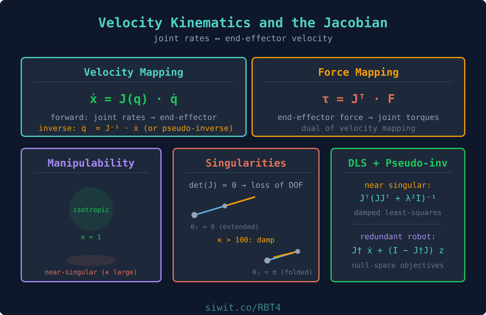
The Jacobian matrix maps joint velocities to end-effector velocities through
Forward velocity mapping is always straightforward (matrix multiplication)
Inverse velocity mapping requires (square) or (redundant) and fails at singularities
Singularities occur when ; for the 2R robot, this means
Manipulability ellipsoids (from SVD) visualize directional velocity capability
Pseudoinverse gives the minimum-norm solution for redundant robots, with null-space freedom for secondary objectives
Force mapping uses and is the dual of velocity mapping
Collaborative safety requires continuous Jacobian-based force monitoring, especially near singularities

What Comes Next

In Lesson 5, we will build on the Jacobian to plan smooth trajectories in both joint space and task space, using polynomial interpolation and velocity profiles to execute pick-and-place operations with the collaborative robot.

Comments

Loading comments...