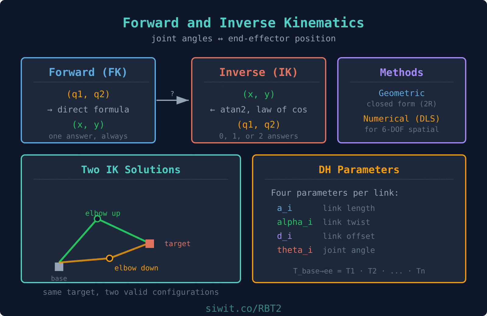
Forward and inverse kinematics are the two central problems in robotic manipulation. Forward kinematics (FK) maps joint angles to end-effector position, answering “where is the tool?” Inverse kinematics (IK) reverses the question: “what joint angles place the tool at this target?” This lesson develops both frameworks through a robotic welding application, using geometric closed-form solutions and numerical iteration for when closed-form methods break down. #ForwardKinematics #InverseKinematics #RoboticWelding
Learning Objectives
By the end of this lesson, you will be able to:
Derive forward kinematics equations for planar 2R and 3R robot arms using trigonometry and transformation matrices
Apply Denavit-Hartenberg (DH) parameter conventions to systematically build FK solutions for serial manipulators
Solve inverse kinematics using geometric (closed-form) methods for 2R planar robots
Identify multiple IK solutions (elbow-up vs. elbow-down) and select the appropriate configuration for a given task
Implement numerical IK using Jacobian-based Newton-Raphson iteration for robots without closed-form solutions
Analyze workspace boundaries, singularities, and unreachable positions
Real-World Engineering Challenge: Robotic Welding of Curved Seams
A 2-DOF planar robot arm is tasked with welding a curved seam on a cylindrical pressure vessel. The seam follows an arc defined by discrete waypoints along the vessel surface. The robot must position its welding torch at each waypoint with millimeter-level accuracy. The arm has link lengths mm and mm, and the weld seam lies partially near the boundary of the robot’s reachable workspace. The production line requires the robot to complete each weld pass in under 8 seconds, so joint angle computation must be fast and reliable.
Why This Problem Matters in Industry
Robotic welding is one of the largest applications of industrial manipulators. Automotive body shops, shipbuilding, pipeline construction, and pressure vessel fabrication all rely on robots to follow complex seam geometries at consistent speed and heat input. The kinematic accuracy of the robot directly affects weld quality: too much positional error causes incomplete fusion, porosity, or burn-through. Forward kinematics provides the feedback loop (verifying where the torch actually is), while inverse kinematics drives the control loop (commanding where the torch needs to go). Together, they form the computational backbone of every robotic welding cell.
Forward Kinematics: From Joint Angles to End-Effector Position
Forward kinematics answers the question: given all joint angles , where is the end-effector in Cartesian space? For serial manipulators, the answer is built by chaining coordinate transformations from the base frame through each link to the tool frame. We begin with the simplest case, a 2R planar robot, then extend the approach to general serial chains using DH parameters.
FK for a 2R Planar Robot
  2R Planar Robot Arm
                          end-effector (x_e, y_e)                         /                        / Link 2 (L2)                       /              elbow --+  angle theta2             (x1,y1) /   (relative to Link 1)                     /                    / Link 1 (L1)                   /                  / angle theta1  base (0,0) ---+  (from +x axis)                 -----------> x
Consider a planar robot with two revolute joints. Link 1 has length and rotates by angle from the horizontal. Link 2 has length and rotates by angle relative to link 1.
The position of the elbow joint (end of link 1) is:
The position of the end-effector (end of link 2) is:
These two equations are the complete FK solution for a 2R planar arm. Given any pair , we can compute directly.
FK Implementation in Python
import numpy as np
import matplotlib.pyplot as plt
defforward_kinematics_2R(L1, L2, theta1, theta2):
"""Compute end-effector position for a 2R planar robot.
Args:
L1: Length of link 1 (mm)
L2: Length of link 2 (mm)
theta1: Joint 1 angle (radians), measured from +x axis
theta2: Joint 2 angle (radians), relative to link 1
Returns:
(x_e, y_e): End-effector position in base frame (mm)
(x_1, y_1): Elbow position in base frame (mm)
"""
# Elbow (joint 2) position
x1 = L1 * np.cos(theta1)
y1 = L1 * np.sin(theta1)
# End-effector position
x_e = x1 + L2 * np.cos(theta1 + theta2)
y_e = y1 + L2 * np.sin(theta1 + theta2)
return (x_e, y_e), (x1, y1)
# Example: L1 = 400mm, L2 = 300mm
L1, L2 =400, 300
theta1 = np.radians(45) # 45 degrees
theta2 = np.radians(-30) # -30 degrees relative to link 1
For robots with more than two or three joints, writing out FK equations by hand becomes error-prone. The Denavit-Hartenberg convention provides a systematic way to assign coordinate frames to each link and express the transformation between consecutive frames using exactly four parameters. If you need a refresher on homogeneous transformation matrices and how they compose, see Elementary Matrix Methods and Link Modeling.
  DH Frame Assignment (two consecutive frames)
  z_{i-1}                          z_i    |                                |    |  d_i (offset along z_{i-1})   |    |  |                             |    |  v                             |    +---------> x_{i-1}             +---------> x_i   frame i-1                       frame i              |<--- a_i (link length along x_i) --->|
  alpha_i = angle from z_{i-1} to z_i, measured about x_i  theta_i = angle from x_{i-1} to x_i, measured about z_{i-1}
Each link in a serial chain is described by four DH parameters:
Parameter
Symbol
Description
Link length
Distance along from to
Link twist
Angle about from to
Link offset
Distance along from to
Joint angle
Angle about from to
For a revolute joint, is the variable. For a prismatic joint, is the variable. The remaining parameters are constants determined by the robot geometry.
The transformation matrix from frame to frame is:
The overall FK from base to end-effector is the product of all individual transformations:
defdh_transform(theta, d, a, alpha):
"""Compute the 4x4 DH transformation matrix.
Args:
theta: Joint angle (rad)
d: Link offset (mm)
a: Link length (mm)
alpha: Link twist (rad)
Returns:
4x4 numpy array (homogeneous transformation)
"""
ct, st = np.cos(theta), np.sin(theta)
ca, sa = np.cos(alpha), np.sin(alpha)
return np.array([
[ct, -st * ca, st * sa, a * ct],
[st, ct * ca, -ct * sa, a * st],
[0, sa, ca, d ],
[0, 0, 0, 1]
])
deffk_from_dh(dh_table, joint_angles):
"""Compute FK from a DH parameter table.
Args:
dh_table: List of (a, alpha, d, theta_offset) for each joint
joint_angles: List of joint angle values (rad)
Returns:
4x4 homogeneous transformation (base to end-effector)
"""
T = np.eye(4)
for i, (a, alpha, d, theta_offset) inenumerate(dh_table):
theta = joint_angles[i] + theta_offset
T = T @dh_transform(theta, d, a, alpha)
return T
# DH table for 2R planar robot
# (a, alpha, d, theta_offset)
dh_2R =[
(400, 0, 0, 0), # Link 1: a=400mm, planar
(300, 0, 0, 0), # Link 2: a=300mm, planar
]
# Test: same angles as before
q =[np.radians(45), np.radians(-30)]
T =fk_from_dh(dh_2R, q)
print(f"End-effector position from DH: ({T[0,3]:.1f}, {T[1,3]:.1f}) mm")
DH parameters for common industrial robots
Most 6-DOF industrial robots (such as the ABB IRB series, KUKA KR series, or Fanuc M-series) use a standard anthropomorphic configuration with three intersecting axes at the wrist. The first three joints position the wrist center, and the last three orient the tool. This “spherical wrist” structure enables a decoupled IK solution: position IK for joints 1 through 3, then orientation IK for joints 4 through 6. The DH parameters for each specific robot model are published in the manufacturer’s technical documentation.
Inverse Kinematics: From Target Position to Joint Angles
Inverse kinematics is the harder of the two problems. Given a desired end-effector position , we need to find joint angles that place the end-effector there. Unlike FK, IK can have zero solutions (target unreachable), exactly one solution (target on workspace boundary), or multiple solutions (interior of workspace). The two main approaches are geometric (closed-form) and numerical (iterative).
Numerical Inverse Kinematics Using Newton-Raphson Iteration
Geometric IK works beautifully for simple planar robots, but it does not scale to 6-DOF spatial manipulators or robots with complex joint configurations. Numerical IK uses iterative optimization to converge on a solution. The most common approach is the Jacobian-based Newton-Raphson method, which linearizes the FK mapping at each step and solves a linear system to update the joint angles.
The Algorithm:
Start with an initial guess for the joint angles.
Compute the current end-effector position using FK: .
Compute the position error: .
If (tolerance), stop. The solution is .
Compute the Jacobian matrix at the current configuration.
Solve for the joint angle update: (or use the pseudoinverse for non-square systems).
Update: .
Repeat from step 2.
The Jacobian matrix for a 2R planar robot relates joint velocities to end-effector velocity:
From the FK equations:
defjacobian_2R(L1, L2, theta1, theta2):
"""Compute the 2x2 Jacobian for a 2R planar robot.
Args:
L1, L2: Link lengths (mm)
theta1, theta2: Joint angles (rad)
Returns:
2x2 numpy array (Jacobian matrix)
"""
s1 = np.sin(theta1)
c1 = np.cos(theta1)
s12 = np.sin(theta1 + theta2)
c12 = np.cos(theta1 + theta2)
J = np.array([
[-L1 * s1 - L2 * s12, -L2 * s12],
[ L1 * c1 + L2 * c12, L2 * c12]
])
return J
defnumerical_ik_2R(L1, L2, x_t, y_t,
q0=None, tol=1e-6, max_iter=100,
damping=1e-4):
"""Numerical IK using damped Jacobian iteration.
Args:
L1, L2: Link lengths (mm)
x_t, y_t: Target position (mm)
q0: Initial joint angle guess (rad). Defaults to [0.5, 0.5].
tol: Convergence tolerance (mm)
max_iter: Maximum iterations
damping: Damping factor for singularity robustness
Returns:
(theta1, theta2): Joint angles (rad), or None if no convergence
The numerical IK result depends on the initial guess. Different starting configurations converge to different valid solutions (or may fail to converge altogether). This is both a feature and a challenge: you can steer the solver toward a preferred configuration (e.g., elbow-up) by choosing an appropriate initial guess, but you must be aware that the solver may find an unexpected configuration if the guess is poor.
# Demonstrate that different initial guesses yield different solutions
The workspace of a robot is the set of all points the end-effector can reach. For a 2R planar robot, the workspace is an annular region (a ring) between two concentric circles. The outer boundary has radius (arm fully extended). The inner boundary has radius (arm fully folded back). If , the inner boundary collapses to a single point at the origin, and the entire disk is reachable.
We now return to the original welding challenge and apply both FK and IK to trace a curved seam path. The seam is defined as a sequence of waypoints along an arc on the pressure vessel surface. The robot must compute joint angles for each waypoint, check reachability, select the appropriate elbow configuration for smooth motion, and verify the path before execution.
After computing joint angles from IK, run them back through FK to confirm the end-effector lands at the target. Round-trip verification catches numerical errors, especially near workspace boundaries where small angle changes produce large position shifts.
Choose Elbow Configuration Deliberately
For continuous path following (welding, painting, gluing), maintain a consistent elbow configuration throughout the trajectory. Switching between elbow-up and elbow-down mid-path causes discontinuous joint motion and may damage the workpiece or the robot.
Avoid Workspace Boundaries
Near the outer boundary (), joint velocities spike because small Cartesian displacements require large joint angle changes. Plan paths with at least 5-10% margin from the workspace limits. If a waypoint must be near the boundary, reduce the Cartesian velocity for that segment.
Use Damped Least-Squares for Numerical IK
The standard Jacobian inverse fails at singular configurations ( or ). The damped least-squares (Levenberg-Marquardt) method adds a small regularization term to , trading off accuracy for stability. Typical damping values range from to .
Initial Guess Strategy
For trajectory following, use the previous waypoint’s solution as the initial guess for the next waypoint. This exploits the continuity of the path and typically converges in 2 to 4 iterations. For the first point, use a known home configuration or a random guess within expected joint limits.
Handle Unreachable Points Gracefully
In production systems, the path planner must detect unreachable waypoints before execution begins. Options include repositioning the robot base, splitting the task across multiple setups, or using a robot with longer reach. Never allow the controller to attempt IK on an unreachable target without a fallback strategy.
Check Joint Limits After IK
The geometric IK function above returns mathematically valid angles but does not know about your robot’s joint limits. A target can be inside the reachable workspace and still require a joint angle outside [theta_min, theta_max]. Wrap every IK call with a limit check:
for (t1, t2) in solutions:
if (theta1_min <= t1 <= theta1_max
and theta2_min <= t2 <= theta2_max):
# use this solution
If no solution satisfies the limits, the target is unreachable in practice even though it is inside the ideal workspace.
Be Consistent About Units
The examples here use millimeters for link lengths and radians for joint angles. Mixing unit systems is a classic bug source: passing degrees into np.cos, or millimeters into a function expecting meters. Pick one convention per codebase, document it at the module level, and convert only at the interface with the UI or hardware driver. Angles should travel as radians through every internal function.
Summary
This lesson covered the two fundamental kinematic problems in robotics. Forward kinematics computes end-effector position from joint angles using either direct trigonometric equations or the systematic DH parameter framework. For the 2R planar robot, the FK equations are simple: and . Inverse kinematics reverses this mapping. The geometric approach yields closed-form solutions using the law of cosines and atan2, producing two solutions (elbow-up and elbow-down) for interior workspace points. The numerical Jacobian-based approach handles arbitrary robot configurations through iterative refinement, with damped least-squares providing robustness near singularities. Both methods were applied to a robotic welding application, demonstrating path planning, reachability checking, and configuration selection for smooth seam following.
Next lesson:Orientation and Quaternions extends kinematic analysis to 3D rotations, covering Euler angles, gimbal lock, quaternion math, and SLERP interpolation for smooth orientation control.
Comments