Real-Time Systems Concepts

Modified: Mar. 14, 2026

Published: Jan. 24, 2026

Every embedded system makes promises about timing. A motor controller must update its PWM output within microseconds, a sensor logger must sample at a fixed rate, and a safety interlock must respond before a mechanical limit is reached. In this lesson you will build a jitter measurement rig that toggles GPIO pins from both a bare-metal super loop and a FreeRTOS task, then compare the timing stability of each approach on an oscilloscope or logic analyzer. The results will show you exactly why real-time operating systems exist. #RTOS #RealTime #Jitter

What We Are Building

Jitter Measurement Rig

A side-by-side timing comparison between bare-metal and RTOS task execution. Two GPIO pins toggle at a target frequency: one driven by a simple while-loop delay, the other by a FreeRTOS periodic task. You will capture both signals, measure jitter, and calculate worst-case execution time for each approach.

Project specifications:

Parameter	Value
MCU	STM32 Blue Pill (STM32F103C8T6) or ESP32 DevKit
RTOS	FreeRTOS (bundled with ESP-IDF or STM32CubeMX)
Target toggle rate	1 kHz (1 ms period)
Measurement	GPIO jitter via logic analyzer or oscilloscope
Indicator	LED on bare-metal pin, LED on RTOS pin
Key metrics	Mean period, standard deviation, worst-case jitter
Components	MCU board, 1 LED, jumper wires, logic analyzer (optional)

Parts List

Ref	Component	Quantity	Notes
U1	STM32 Blue Pill or ESP32 DevKit	1	Reuse from prior courses
D1	LED (any color)	1	Visual toggle indicator
R1	330 ohm resistor	1	LED current limiter
J1	Logic analyzer	1	Optional, for precise jitter capture
-	Jumper wires	Several	For breadboard connections

What Is Real-Time?

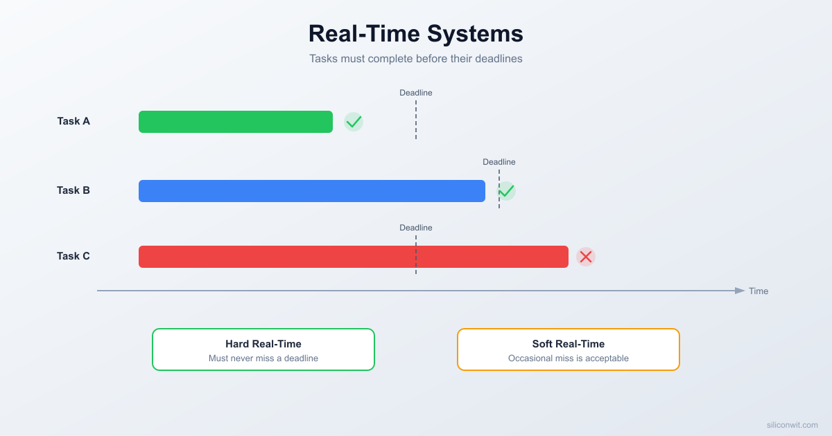
A system is “real-time” when correctness depends not only on producing the right answer but on producing it before a deadline. A sorting algorithm that returns the correct result one second late is still correct in a general-purpose context. A brake controller that commands the calipers one second late is a failure, regardless of how mathematically perfect the output is.

Real-time systems are classified into three categories based on the consequences of missing a deadline.

Hard Real-Time

A missed deadline is a system failure. The result produced after the deadline is not just late; it is dangerous or useless. Examples include airbag deployment controllers, anti-lock brake modules, cardiac pacemakers, and motor commutation loops. These systems must guarantee that every deadline is met under all operating conditions.

Soft Real-Time

A missed deadline degrades quality but does not cause failure. The system continues to function, and late results still have value. Audio and video streaming are classic examples: a dropped frame or a glitch in the audio is noticeable but tolerable. The system recovers on the next cycle. Most interactive user interfaces also fall into this category.

Firm Real-Time

A late result is worthless but does not cause catastrophic failure. The system simply discards the result and moves on. A sensor sampling system that misses its window produces stale data that cannot be used in the current control cycle, but the hardware is not damaged. Financial trading systems that must execute within a price window are another example: a late trade is not executed, but nothing crashes.

Category	Missed Deadline Consequence	Example
Hard	System failure or safety hazard	Airbag controller, motor commutation
Soft	Degraded quality, system recovers	Audio streaming, GUI updates
Firm	Late result discarded, no damage	Sensor sampling, network packet processing

Most embedded systems you will build in practice fall into the soft or firm category. True hard real-time systems require formal verification, certified toolchains, and exhaustive testing. The techniques in this lesson (jitter measurement, WCET analysis, rate-monotonic scheduling) apply to all three categories, but they are essential for hard real-time work.

 Deadline Severity Spectrum
 ─────────────────────────────────────────────
  Soft               Firm              Hard
  (degraded          (result           (system
   quality)           discarded)        failure)

  Audio stream       Sensor sample     Airbag
  GUI refresh        Packet timeout    Pacemaker
  Video frame        Price window      Motor ctrl

  ◄── tolerable ──► ◄── useless ──► ◄── danger ──►
  if late             if late           if late
 ─────────────────────────────────────────────

The Super-Loop Problem

If you completed the STM32 or ESP32 courses, every project used the same fundamental structure: a while(1) loop in main() that calls each task function in sequence.

int main(void) {
    system_init();

    while (1) {
        read_temperature_sensor();   // ~2 ms
        update_lcd_display();        // ~8 ms
        check_button_inputs();       // ~0.1 ms
        send_serial_report();        // ~3 ms
    }
}

This is called a super loop (or polling loop, or bare-metal loop). It is simple, requires no OS, and works well for many applications. But it has a fundamental timing problem.

The loop period is the sum of all task execution times. In the example above, one full iteration takes roughly 2 + 8 + 0.1 + 3 = 13.1 ms. The temperature sensor is read once every 13.1 ms. If you add a new function that takes 5 ms, the sensor now waits 18.1 ms between reads. Every task in the loop is affected by every other task.

  Super Loop Timing (each task blocks all others)
  ──────────────────────────────────────────────
  │  read_temp  │update_lcd │ btn │ serial │
  │    2 ms     │   8 ms    │0.1ms│  3 ms  │
  ├─────────────┼───────────┼─────┼────────┤
  0            2           10   10.1      13.1 ms
  │◄──────── one loop iteration ─────────►│

  If update_lcd grows to 12 ms:
  │  read_temp  │  update_lcd   │ btn │serial│
  │    2 ms     │    12 ms      │0.1ms│ 3 ms │
  ├─────────────┼───────────────┼─────┼──────┤
  0            2              14   14.1    17.1 ms
  Loop period grew by 4 ms. Every task affected.

This coupling creates jitter: variation in the time between successive executions of the same function. If update_lcd_display() sometimes takes 8 ms and sometimes takes 12 ms (because of conditional rendering), the sensor read interval varies by 4 ms, and the serial report interval varies by the same amount. No task can maintain a stable period independent of the others.

For a blinking LED this does not matter. For a PID motor controller that expects a fixed sample rate, or a communication protocol with tight timing windows, jitter can cause instability, data corruption, or missed packets.

Measuring Jitter: Bare-Metal

The most reliable way to observe jitter is to toggle a GPIO pin at a known target interval and capture the output with an oscilloscope or logic analyzer. The variation in the measured period is your jitter.

Here is a bare-metal program that attempts to toggle PA0 every 1 ms:

STM32 (Blue Pill)
ESP32 (ESP-IDF)

/* bare_metal_jitter.c - STM32 Blue Pill */
#include "stm32f1xx_hal.h"

void SystemClock_Config(void);
static void GPIO_Init(void);
void simulate_sensor_read(void);

int main(void) {
    HAL_Init();
    SystemClock_Config();
    GPIO_Init();

    uint32_t last_tick = HAL_GetTick();

    while (1) {
        /* Wait until 1 ms has elapsed */
        while ((HAL_GetTick() - last_tick) < 1) {
            /* spin */
        }
        last_tick += 1;

        /* Toggle PA0 - this is the pin we measure */
        HAL_GPIO_TogglePin(GPIOA, GPIO_PIN_0);

        /* Simulate other work in the super loop */
        simulate_sensor_read();
    }
}

void simulate_sensor_read(void) {
    /* Busy wait ~200 us at 72 MHz */
    volatile uint32_t count = 3600;
    while (count--) { }
}

static void GPIO_Init(void) {
    __HAL_RCC_GPIOA_CLK_ENABLE();

    GPIO_InitTypeDef gpio = {0};
    gpio.Pin   = GPIO_PIN_0;
    gpio.Mode  = GPIO_MODE_OUTPUT_PP;
    gpio.Speed = GPIO_SPEED_FREQ_HIGH;
    HAL_GPIO_Init(GPIOA, &gpio);
}

/* bare_metal_jitter.c - ESP32 */
#include <stdio.h>
#include "driver/gpio.h"
#include "esp_timer.h"
#include "rom/ets_sys.h"

#define TOGGLE_PIN  GPIO_NUM_2

void simulate_sensor_read(void);

void app_main(void) {
    gpio_reset_pin(TOGGLE_PIN);
    gpio_set_direction(TOGGLE_PIN, GPIO_MODE_OUTPUT);

    int64_t last_time = esp_timer_get_time();  /* microseconds */

    while (1) {
        /* Wait until 1000 us (1 ms) has elapsed */
        while ((esp_timer_get_time() - last_time) < 1000) {
            /* spin */
        }
        last_time += 1000;

        gpio_set_level(TOGGLE_PIN, !gpio_get_level(TOGGLE_PIN));

        /* Simulate other work */
        simulate_sensor_read();
    }
}

void simulate_sensor_read(void) {
    ets_delay_us(200);
}

Connect your logic analyzer or oscilloscope probe to PA0 (or GPIO2 on the ESP32) and GND. You should see a square wave with a period close to 2 ms (toggle every 1 ms means the full cycle is 2 ms).

Now increase the sensor simulation to 800 us:

void simulate_sensor_read(void) {
    /* ~800 us busy wait at 72 MHz */
    volatile uint32_t count = 14400;
    while (count--) { }
}

The toggle still tries to fire every 1 ms, but the sensor work takes 800 us, leaving only 200 us of margin. If any interrupt or other overhead pushes the total past 1 ms, the toggle slips. On the logic analyzer you will see the period stretch beyond 2 ms. This is bare-metal jitter in action: the timing of every task is coupled to the execution time of every other task in the loop.

FreeRTOS in 60 Seconds

FreeRTOS solves the super-loop coupling problem by giving each task its own context (stack, program counter, registers) and letting a scheduler decide which task runs at any given moment. The scheduler is driven by a periodic hardware interrupt called the tick interrupt.

Key concepts:

Task: an independent function with its own stack that runs as if it owns the CPU. Each task has a priority level.
Scheduler: runs on every tick interrupt. It checks which tasks are ready and switches the CPU to the highest-priority ready task.
Tick interrupt: fires at configTICK_RATE_HZ (typically 1000 Hz, giving a 1 ms tick). This is the heartbeat of the RTOS.
Preemption: if a higher-priority task becomes ready (for example, its delay expires), the scheduler immediately pauses the current task and switches to the higher-priority one. The paused task resumes later exactly where it left off.

Adding FreeRTOS to an STM32 Project

If you use STM32CubeMX, enable CMSIS_V2 under Middleware and FreeRTOS. CubeMX generates the FreeRTOS source files and configuration header. If you prefer a manual setup, download the FreeRTOS kernel source, add the portable layer for ARM Cortex-M3 (portable/GCC/ARM_CM3), and include FreeRTOSConfig.h in your project.

On ESP32, FreeRTOS is built into ESP-IDF. You do not need to add anything; just include freertos/FreeRTOS.h and freertos/task.h.

Creating a Task

void my_task(void *params) {
    while (1) {
        /* do work */
        vTaskDelay(pdMS_TO_TICKS(100));  /* sleep 100 ms */
    }
}

/* In main or app_main: */
xTaskCreate(
    my_task,        /* task function */
    "MyTask",       /* name (for debugging) */
    256,            /* stack size in words */
    NULL,           /* parameter passed to task */
    2,              /* priority (higher number = higher priority) */
    NULL            /* task handle (optional) */
);

vTaskStartScheduler();  /* STM32 only; ESP-IDF starts it automatically */

The call to vTaskStartScheduler() hands control to FreeRTOS. On STM32 you call it at the end of main(). On ESP32 the scheduler is already running when app_main() is called, so you only need xTaskCreate.

Measuring Jitter: FreeRTOS

Now let us repeat the jitter experiment, but this time the GPIO toggle runs inside a FreeRTOS periodic task using vTaskDelayUntil(). This function sleeps until an absolute tick count, not for a relative duration, so the period is independent of how long the task body takes to execute.

STM32 (Blue Pill)
ESP32 (ESP-IDF)

/* rtos_jitter.c - STM32 Blue Pill with FreeRTOS */
#include "stm32f1xx_hal.h"
#include "FreeRTOS.h"
#include "task.h"

static void GPIO_Init(void);

void toggle_task(void *params) {
    TickType_t xLastWakeTime = xTaskGetTickCount();

    while (1) {
        HAL_GPIO_TogglePin(GPIOA, GPIO_PIN_0);
        vTaskDelayUntil(&xLastWakeTime, pdMS_TO_TICKS(1));
    }
}

void sensor_task(void *params) {
    while (1) {
        /* Simulate 800 us of sensor work */
        volatile uint32_t count = 14400;
        while (count--) { }
        vTaskDelay(pdMS_TO_TICKS(5));
    }
}

int main(void) {
    HAL_Init();
    SystemClock_Config();
    GPIO_Init();

    xTaskCreate(toggle_task, "Toggle", 128, NULL, 3, NULL);
    xTaskCreate(sensor_task, "Sensor", 128, NULL, 1, NULL);

    vTaskStartScheduler();

    while (1) { }  /* should never reach here */
}

/* rtos_jitter.c - ESP32 with FreeRTOS */
#include <stdio.h>
#include "freertos/FreeRTOS.h"
#include "freertos/task.h"
#include "driver/gpio.h"

#define TOGGLE_PIN  GPIO_NUM_2

void toggle_task(void *params) {
    TickType_t xLastWakeTime = xTaskGetTickCount();

    while (1) {
        gpio_set_level(TOGGLE_PIN, !gpio_get_level(TOGGLE_PIN));
        vTaskDelayUntil(&xLastWakeTime, pdMS_TO_TICKS(1));
    }
}

void sensor_task(void *params) {
    while (1) {
        /* Simulate 800 us of sensor work */
        ets_delay_us(800);
        vTaskDelay(pdMS_TO_TICKS(5));
    }
}

void app_main(void) {
    gpio_reset_pin(TOGGLE_PIN);
    gpio_set_direction(TOGGLE_PIN, GPIO_MODE_OUTPUT);

    xTaskCreate(toggle_task, "Toggle", 2048, NULL, 5, NULL);
    xTaskCreate(sensor_task, "Sensor", 2048, NULL, 1, NULL);
}

Flash this and capture PA0 on the logic analyzer. The toggle period will be rock-solid at 2 ms (1 ms per toggle), even though the sensor task is burning 800 us of CPU time every 5 ms. The scheduler preempts the sensor task whenever the toggle task’s delay expires, so the toggle task runs at its target rate regardless of what else is happening.

This is the core value proposition of an RTOS: tasks with different periods and priorities run independently. Adding more low-priority work does not affect the timing of high-priority tasks.

Worst-Case Execution Time (WCET)

Knowing the average execution time of a function is not enough for real-time systems. You need the worst-case execution time (WCET): the longest time the function will ever take to complete under any possible input and system state.

Why is average-case dangerous? Consider a function that usually takes 50 us but occasionally takes 500 us when a particular branch condition is met. If you design your schedule based on the 50 us average, the system will miss deadlines whenever the slow path triggers. In a hard real-time system, that single miss can be catastrophic.

Measuring WCET

The practical approach is to toggle a GPIO pin high at the start of the critical code section and low at the end, then capture the signal with a logic analyzer over thousands of iterations.

void critical_function(void) {
    HAL_GPIO_WritePin(GPIOA, GPIO_PIN_1, GPIO_PIN_SET);   /* probe high */

    /* --- critical code under test --- */
    process_sensor_data();
    compute_pid_output();
    update_pwm();
    /* --- end critical code --- */

    HAL_GPIO_WritePin(GPIOA, GPIO_PIN_1, GPIO_PIN_RESET); /* probe low */
}

On your logic analyzer, measure the pulse width (high time) across all captured cycles. The maximum pulse width is your measured WCET. For safety, add a margin of 10 to 20 percent on top of the measured maximum to account for rare cache misses, flash wait states, or interrupt latency that you may not have triggered during testing.

Static analysis tools (such as aiT or Bound-T) can compute WCET from the binary without running the code, but they require detailed hardware models and are typically used only in safety-critical industries (automotive, aerospace, medical).

Rate-Monotonic Analysis (RMA)

Once you know the WCET of each task, you can use Rate-Monotonic Analysis to determine whether a set of periodic tasks is schedulable, meaning all tasks will always meet their deadlines.

The Rule

Assign the highest priority to the task with the shortest period. This is the rate-monotonic priority assignment, and it is provably optimal for fixed-priority preemptive scheduling of independent periodic tasks.

  Rate-Monotonic Priority Assignment
  ───────────────────────────────────
  Shortest period  ──►  Highest priority

  Task       Period    Priority
  ─────────  ──────    ────────
  Toggle LED   1 ms    3 (highest)
  Read sensor  5 ms    2
  Send report 20 ms    1 (lowest)

The Utilization Bound Test

For N periodic tasks, each with a worst-case execution time and period , calculate the total CPU utilization:

The task set is guaranteed schedulable if:

For common values of N:

N (tasks)	Utilization Bound
1	1.000 (100%)
2	0.828 (82.8%)
3	0.780 (78.0%)
4	0.757 (75.7%)
Infinity	0.693 (69.3%)

Worked Example

Suppose you have three periodic tasks:

Task	Period ()	WCET ()	Utilization ()
Toggle LED	1 ms	0.01 ms	0.010
Read sensor	5 ms	0.80 ms	0.160
Send report	20 ms	2.00 ms	0.100

Total utilization:

The bound for 3 tasks is 0.780. Since , the task set is schedulable with rate-monotonic priority assignment (Toggle LED gets the highest priority because it has the shortest period).

Now suppose you add a heavy processing task with a period of 10 ms and WCET of 6 ms:

The bound for 4 tasks is 0.757. Since , the utilization test fails. This does not guarantee a deadline miss (the test is sufficient but not necessary), but it is a strong warning that the task set may not be schedulable. You would need to either reduce the processing time, increase the period, or use a more detailed analysis (response time analysis) to determine schedulability.

Complete Project: Jitter Measurement Rig

This project creates three FreeRTOS tasks at different priorities, toggles GPIO pins in the two periodic tasks, and prints jitter statistics over serial. You can observe the toggles on a logic analyzer and confirm the numbers match the serial output.

STM32 (Blue Pill)
ESP32 (ESP-IDF)

/* main.c - Jitter Measurement Rig (STM32 Blue Pill + FreeRTOS) */

#include "stm32f1xx_hal.h"
#include "FreeRTOS.h"
#include "task.h"
#include <stdio.h>
#include <string.h>

/* ---------- Hardware configuration ---------- */
static UART_HandleTypeDef huart1;

static void SystemClock_Config(void);
static void GPIO_Init(void);
static void UART_Init(void);
static void uart_print(const char *msg);

/* ---------- Jitter tracking ---------- */
typedef struct {
    uint32_t min_period_us;
    uint32_t max_period_us;
    uint32_t sum_period_us;
    uint32_t count;
    uint32_t last_tick_us;
} JitterStats;

static volatile JitterStats stats_1ms = { .min_period_us = UINT32_MAX };
static volatile JitterStats stats_5ms = { .min_period_us = UINT32_MAX };

/* Microsecond timestamp using DWT cycle counter */
static inline uint32_t get_us(void) {
    return DWT->CYCCNT / (SystemCoreClock / 1000000);
}

static void dwt_init(void) {
    CoreDebug->DEMCR |= CoreDebug_DEMCR_TRCENA_Msk;
    DWT->CYCCNT = 0;
    DWT->CTRL |= DWT_CTRL_CYCCNTENA_Msk;
}

/* ---------- Task 1: Toggle PA0 every 1 ms (high priority) ---------- */
void task_toggle_1ms(void *params) {
    TickType_t xLastWakeTime = xTaskGetTickCount();

    /* Prime the timestamp */
    stats_1ms.last_tick_us = get_us();

    while (1) {
        vTaskDelayUntil(&xLastWakeTime, pdMS_TO_TICKS(1));

        uint32_t now = get_us();
        uint32_t elapsed = now - stats_1ms.last_tick_us;
        stats_1ms.last_tick_us = now;

        if (stats_1ms.count > 0) {  /* skip first sample */
            if (elapsed < stats_1ms.min_period_us)
                stats_1ms.min_period_us = elapsed;
            if (elapsed > stats_1ms.max_period_us)
                stats_1ms.max_period_us = elapsed;
            stats_1ms.sum_period_us += elapsed;
        }
        stats_1ms.count++;

        HAL_GPIO_TogglePin(GPIOA, GPIO_PIN_0);
    }
}

/* ---------- Task 2: Toggle PA1 every 5 ms (medium priority) ---------- */
void task_toggle_5ms(void *params) {
    TickType_t xLastWakeTime = xTaskGetTickCount();

    stats_5ms.last_tick_us = get_us();

    while (1) {
        vTaskDelayUntil(&xLastWakeTime, pdMS_TO_TICKS(5));

        uint32_t now = get_us();
        uint32_t elapsed = now - stats_5ms.last_tick_us;
        stats_5ms.last_tick_us = now;

        if (stats_5ms.count > 0) {
            if (elapsed < stats_5ms.min_period_us)
                stats_5ms.min_period_us = elapsed;
            if (elapsed > stats_5ms.max_period_us)
                stats_5ms.max_period_us = elapsed;
            stats_5ms.sum_period_us += elapsed;
        }
        stats_5ms.count++;

        HAL_GPIO_TogglePin(GPIOA, GPIO_PIN_1);
    }
}

/* ---------- Task 3: Simulate sensor work (low priority) ---------- */
void task_sensor_work(void *params) {
    while (1) {
        /* Busy loop simulating 800 us of ADC + filtering work */
        volatile uint32_t count = 14400;
        while (count--) { }

        vTaskDelay(pdMS_TO_TICKS(2));
    }
}

/* ---------- Task 4: Print statistics every 2 seconds ---------- */
void task_report(void *params) {
    char buf[128];

    while (1) {
        vTaskDelay(pdMS_TO_TICKS(2000));

        if (stats_1ms.count > 2) {
            uint32_t mean = stats_1ms.sum_period_us / (stats_1ms.count - 1);
            snprintf(buf, sizeof(buf),
                "1ms task: min=%lu us, max=%lu us, mean=%lu us, jitter=%lu us\r\n",
                (unsigned long)stats_1ms.min_period_us,
                (unsigned long)stats_1ms.max_period_us,
                (unsigned long)mean,
                (unsigned long)(stats_1ms.max_period_us - stats_1ms.min_period_us));
            uart_print(buf);
        }

        if (stats_5ms.count > 2) {
            uint32_t mean = stats_5ms.sum_period_us / (stats_5ms.count - 1);
            snprintf(buf, sizeof(buf),
                "5ms task: min=%lu us, max=%lu us, mean=%lu us, jitter=%lu us\r\n",
                (unsigned long)stats_5ms.min_period_us,
                (unsigned long)stats_5ms.max_period_us,
                (unsigned long)mean,
                (unsigned long)(stats_5ms.max_period_us - stats_5ms.min_period_us));
            uart_print(buf);
        }

        uart_print("---\r\n");
    }
}

/* ---------- Main ---------- */
int main(void) {
    HAL_Init();
    SystemClock_Config();
    GPIO_Init();
    UART_Init();
    dwt_init();

    uart_print("Jitter Measurement Rig - Starting FreeRTOS\r\n");

    xTaskCreate(task_toggle_1ms,  "T1ms",   256, NULL, 3, NULL);
    xTaskCreate(task_toggle_5ms,  "T5ms",   256, NULL, 2, NULL);
    xTaskCreate(task_sensor_work, "Sensor",  128, NULL, 1, NULL);
    xTaskCreate(task_report,      "Report",  512, NULL, 1, NULL);

    vTaskStartScheduler();

    /* Should never reach here */
    while (1) { }
}

/* ---------- Peripheral initialization ---------- */
static void GPIO_Init(void) {
    __HAL_RCC_GPIOA_CLK_ENABLE();

    GPIO_InitTypeDef gpio = {0};
    gpio.Pin   = GPIO_PIN_0 | GPIO_PIN_1;
    gpio.Mode  = GPIO_MODE_OUTPUT_PP;
    gpio.Speed = GPIO_SPEED_FREQ_HIGH;
    HAL_GPIO_Init(GPIOA, &gpio);
}

static void UART_Init(void) {
    __HAL_RCC_USART1_CLK_ENABLE();
    __HAL_RCC_GPIOA_CLK_ENABLE();

    GPIO_InitTypeDef gpio = {0};
    gpio.Pin   = GPIO_PIN_9;   /* USART1 TX */
    gpio.Mode  = GPIO_MODE_AF_PP;
    gpio.Speed = GPIO_SPEED_FREQ_HIGH;
    HAL_GPIO_Init(GPIOA, &gpio);

    huart1.Instance          = USART1;
    huart1.Init.BaudRate     = 115200;
    huart1.Init.WordLength   = UART_WORDLENGTH_8B;
    huart1.Init.StopBits     = UART_STOPBITS_1;
    huart1.Init.Parity       = UART_PARITY_NONE;
    huart1.Init.Mode         = UART_MODE_TX;
    huart1.Init.HwFlowCtl    = UART_HWCONTROL_NONE;
    HAL_UART_Init(&huart1);
}

static void uart_print(const char *msg) {
    HAL_UART_Transmit(&huart1, (uint8_t *)msg, strlen(msg), HAL_MAX_DELAY);
}

void SystemClock_Config(void) {
    RCC_OscInitTypeDef osc = {0};
    osc.OscillatorType = RCC_OSCILLATORTYPE_HSE;
    osc.HSEState       = RCC_HSE_ON;
    osc.PLL.PLLState   = RCC_PLL_ON;
    osc.PLL.PLLSource  = RCC_PLLSOURCE_HSE;
    osc.PLL.PLLMUL     = RCC_PLL_MUL9;
    HAL_RCC_OscConfig(&osc);

    RCC_ClkInitTypeDef clk = {0};
    clk.ClockType      = RCC_CLOCKTYPE_HCLK | RCC_CLOCKTYPE_SYSCLK
                        | RCC_CLOCKTYPE_PCLK1 | RCC_CLOCKTYPE_PCLK2;
    clk.SYSCLKSource   = RCC_SYSCLKSOURCE_PLLCLK;
    clk.AHBCLKDivider  = RCC_SYSCLK_DIV1;
    clk.APB1CLKDivider = RCC_HCLK_DIV2;
    clk.APB2CLKDivider = RCC_HCLK_DIV1;
    HAL_RCC_ClockConfig(&clk, FLASH_LATENCY_2);
}

/* main.c - Jitter Measurement Rig (ESP32 + FreeRTOS) */

#include <stdio.h>
#include <string.h>
#include "freertos/FreeRTOS.h"
#include "freertos/task.h"
#include "driver/gpio.h"
#include "esp_timer.h"
#include "rom/ets_sys.h"

#define PIN_1MS   GPIO_NUM_2
#define PIN_5MS   GPIO_NUM_4

/* ---------- Jitter tracking ---------- */
typedef struct {
    uint32_t min_period_us;
    uint32_t max_period_us;
    uint32_t sum_period_us;
    uint32_t count;
    int64_t  last_time_us;
} JitterStats;

static volatile JitterStats stats_1ms = { .min_period_us = UINT32_MAX };
static volatile JitterStats stats_5ms = { .min_period_us = UINT32_MAX };

/* ---------- Task 1: Toggle GPIO2 every 1 ms (high priority) ---------- */
void task_toggle_1ms(void *params) {
    TickType_t xLastWakeTime = xTaskGetTickCount();
    stats_1ms.last_time_us = esp_timer_get_time();

    while (1) {
        vTaskDelayUntil(&xLastWakeTime, pdMS_TO_TICKS(1));

        int64_t now = esp_timer_get_time();
        uint32_t elapsed = (uint32_t)(now - stats_1ms.last_time_us);
        stats_1ms.last_time_us = now;

        if (stats_1ms.count > 0) {
            if (elapsed < stats_1ms.min_period_us)
                stats_1ms.min_period_us = elapsed;
            if (elapsed > stats_1ms.max_period_us)
                stats_1ms.max_period_us = elapsed;
            stats_1ms.sum_period_us += elapsed;
        }
        stats_1ms.count++;

        gpio_set_level(PIN_1MS, !gpio_get_level(PIN_1MS));
    }
}

/* ---------- Task 2: Toggle GPIO4 every 5 ms (medium priority) ---------- */
void task_toggle_5ms(void *params) {
    TickType_t xLastWakeTime = xTaskGetTickCount();
    stats_5ms.last_time_us = esp_timer_get_time();

    while (1) {
        vTaskDelayUntil(&xLastWakeTime, pdMS_TO_TICKS(5));

        int64_t now = esp_timer_get_time();
        uint32_t elapsed = (uint32_t)(now - stats_5ms.last_time_us);
        stats_5ms.last_time_us = now;

        if (stats_5ms.count > 0) {
            if (elapsed < stats_5ms.min_period_us)
                stats_5ms.min_period_us = elapsed;
            if (elapsed > stats_5ms.max_period_us)
                stats_5ms.max_period_us = elapsed;
            stats_5ms.sum_period_us += elapsed;
        }
        stats_5ms.count++;

        gpio_set_level(PIN_5MS, !gpio_get_level(PIN_5MS));
    }
}

/* ---------- Task 3: Simulate sensor work (low priority) ---------- */
void task_sensor_work(void *params) {
    while (1) {
        ets_delay_us(800);
        vTaskDelay(pdMS_TO_TICKS(2));
    }
}

/* ---------- Task 4: Print statistics every 2 seconds ---------- */
void task_report(void *params) {
    while (1) {
        vTaskDelay(pdMS_TO_TICKS(2000));

        if (stats_1ms.count > 2) {
            uint32_t mean = stats_1ms.sum_period_us / (stats_1ms.count - 1);
            printf("1ms task: min=%lu us, max=%lu us, mean=%lu us, jitter=%lu us\n",
                (unsigned long)stats_1ms.min_period_us,
                (unsigned long)stats_1ms.max_period_us,
                (unsigned long)mean,
                (unsigned long)(stats_1ms.max_period_us - stats_1ms.min_period_us));
        }

        if (stats_5ms.count > 2) {
            uint32_t mean = stats_5ms.sum_period_us / (stats_5ms.count - 1);
            printf("5ms task: min=%lu us, max=%lu us, mean=%lu us, jitter=%lu us\n",
                (unsigned long)stats_5ms.min_period_us,
                (unsigned long)stats_5ms.max_period_us,
                (unsigned long)mean,
                (unsigned long)(stats_5ms.max_period_us - stats_5ms.min_period_us));
        }

        printf("---\n");
    }
}

/* ---------- Main ---------- */
void app_main(void) {
    gpio_reset_pin(PIN_1MS);
    gpio_set_direction(PIN_1MS, GPIO_MODE_OUTPUT);
    gpio_reset_pin(PIN_5MS);
    gpio_set_direction(PIN_5MS, GPIO_MODE_OUTPUT);

    printf("Jitter Measurement Rig - Starting tasks\n");

    xTaskCreate(task_toggle_1ms,  "T1ms",   2048, NULL, 5, NULL);
    xTaskCreate(task_toggle_5ms,  "T5ms",   2048, NULL, 3, NULL);
    xTaskCreate(task_sensor_work, "Sensor",  2048, NULL, 1, NULL);
    xTaskCreate(task_report,      "Report",  4096, NULL, 1, NULL);
}

How It Works

The program creates four tasks:

Task	Function	Period	Priority	GPIO Pin
T1ms	Toggle + record jitter	1 ms	3 (high)	PA0 / GPIO2
T5ms	Toggle + record jitter	5 ms	2 (medium)	PA1 / GPIO4
Sensor	Busy loop (simulated work)	2 ms	1 (low)	None
Report	Print statistics over serial	2000 ms	1 (low)	None

The task_toggle_1ms and task_toggle_5ms functions both use vTaskDelayUntil() for precise periodic execution. Each iteration records the elapsed time since the last execution using a microsecond timestamp (DWT cycle counter on STM32, esp_timer_get_time() on ESP32). The minimum, maximum, and sum are tracked to compute jitter and mean period.

The sensor task burns CPU cycles in a busy loop, simulating real ADC and filtering work. Because it runs at the lowest priority, the scheduler preempts it whenever either toggle task is ready to run. This is the key insight: the sensor task consumes spare CPU time without affecting the timing of the higher-priority tasks.

The report task prints statistics every 2 seconds. Typical output looks like:

1ms task: min=999 us, max=1001 us, mean=1000 us, jitter=2 us
5ms task: min=4998 us, max=5002 us, mean=5000 us, jitter=4 us
---

The jitter values of 1 to 4 us are dominated by the tick interrupt resolution and context switch overhead. Compare this to the bare-metal approach where adding 800 us of sensor work can produce jitter in the hundreds of microseconds.

Project Structure

Directoryjitter_measurement_rig/
- Directorysrc/
  - main.c
  - stm32f1xx_hal_conf.h
  - FreeRTOSConfig.h
  - system_stm32f1xx.c
  - startup_stm32f103xb.s
- Directoryinclude/
  - stm32f1xx_hal_conf.h
- Directorylib/
  - DirectoryFreeRTOS/
    DirectorySource/
    tasks.c
    queue.c
    list.c
    Directoryportable/
    DirectoryGCC/
    DirectoryARM_CM3/
    port.c
    portmacro.h
    DirectoryMemMang/
    heap_4.c
    Directoryinclude/
    FreeRTOS.h
    task.h
- Makefile
- STM32F103C8Tx_FLASH.ld

FreeRTOSConfig.h

The most important settings for this project:

#ifndef FREERTOS_CONFIG_H
#define FREERTOS_CONFIG_H

#define configUSE_PREEMPTION              1
#define configUSE_PORT_OPTIMISED_TASK_SELECTION  0
#define configUSE_TICKLESS_IDLE           0
#define configCPU_CLOCK_HZ               (72000000UL)
#define configTICK_RATE_HZ               ((TickType_t)1000)
#define configMAX_PRIORITIES              (5)
#define configMINIMAL_STACK_SIZE         ((uint16_t)128)
#define configTOTAL_HEAP_SIZE            ((size_t)(10 * 1024))
#define configMAX_TASK_NAME_LEN          (16)
#define configUSE_16_BIT_TICKS           0
#define configIDLE_SHOULD_YIELD          1

/* Hook functions */
#define configUSE_IDLE_HOOK              0
#define configUSE_TICK_HOOK              0
#define configCHECK_FOR_STACK_OVERFLOW   2
#define configUSE_MALLOC_FAILED_HOOK     1

/* Co-routine definitions (not used) */
#define configUSE_CO_ROUTINES            0

/* Software timer definitions */
#define configUSE_TIMERS                 0

/* Cortex-M3 interrupt priority configuration */
#define configPRIO_BITS                  4
#define configLIBRARY_LOWEST_INTERRUPT_PRIORITY      15
#define configLIBRARY_MAX_SYSCALL_INTERRUPT_PRIORITY  5
#define configKERNEL_INTERRUPT_PRIORITY       (configLIBRARY_LOWEST_INTERRUPT_PRIORITY << (8 - configPRIO_BITS))
#define configMAX_SYSCALL_INTERRUPT_PRIORITY  (configLIBRARY_MAX_SYSCALL_INTERRUPT_PRIORITY << (8 - configPRIO_BITS))

/* RTOS API includes */
#define INCLUDE_vTaskDelay               1
#define INCLUDE_vTaskDelayUntil          1
#define INCLUDE_vTaskDelete              0
#define INCLUDE_xTaskGetSchedulerState   1
#define INCLUDE_uxTaskGetStackHighWaterMark 1

/* Map FreeRTOS handlers to STM32 interrupt names */
#define vPortSVCHandler     SVC_Handler
#define xPortPendSVHandler  PendSV_Handler
#define xPortSysTickHandler SysTick_Handler

#endif /* FREERTOS_CONFIG_H */

Key points: configTICK_RATE_HZ is set to 1000, giving a 1 ms tick resolution. configUSE_PREEMPTION is enabled so that higher-priority tasks can interrupt lower-priority ones. configCHECK_FOR_STACK_OVERFLOW is set to 2 for maximum stack checking during development.

Makefile

# Makefile for STM32F103 + FreeRTOS (arm-none-eabi-gcc)

TARGET   = jitter_rig
BUILD    = build

CC       = arm-none-eabi-gcc
OBJCOPY  = arm-none-eabi-objcopy
SIZE     = arm-none-eabi-size

# MCU flags
CPU      = -mcpu=cortex-m3 -mthumb
CFLAGS   = $(CPU) -Os -g -Wall -std=c11
CFLAGS  += -DSTM32F103xB -DUSE_HAL_DRIVER
CFLAGS  += -ffunction-sections -fdata-sections

LDFLAGS  = $(CPU) -TSTM32F103C8Tx_FLASH.ld
LDFLAGS += -Wl,--gc-sections -specs=nosys.specs -specs=nano.specs
LDFLAGS += -lc -lm -lnosys

# Include paths
INC  = -Iinclude
INC += -Ilib/FreeRTOS/Source/include
INC += -Ilib/FreeRTOS/Source/portable/GCC/ARM_CM3
INC += -I<path-to-STM32-HAL>/Inc

# Source files
SRC  = src/main.c
SRC += src/system_stm32f1xx.c
SRC += lib/FreeRTOS/Source/tasks.c
SRC += lib/FreeRTOS/Source/queue.c
SRC += lib/FreeRTOS/Source/list.c
SRC += lib/FreeRTOS/Source/portable/GCC/ARM_CM3/port.c
SRC += lib/FreeRTOS/Source/portable/MemMang/heap_4.c

ASM  = src/startup_stm32f103xb.s

OBJ  = $(SRC:%.c=$(BUILD)/%.o) $(ASM:%.s=$(BUILD)/%.o)

all: $(BUILD)/$(TARGET).bin

$(BUILD)/%.o: %.c
  @mkdir -p $(dir $@)
  $(CC) $(CFLAGS) $(INC) -c $< -o $@

$(BUILD)/%.o: %.s
  @mkdir -p $(dir $@)
  $(CC) $(CPU) -c $< -o $@

$(BUILD)/$(TARGET).elf: $(OBJ)
  $(CC) $(LDFLAGS) $^ -o $@
  $(SIZE) $@

$(BUILD)/$(TARGET).bin: $(BUILD)/$(TARGET).elf
  $(OBJCOPY) -O binary $< $@

flash: $(BUILD)/$(TARGET).bin
  openocd -f interface/stlink-v2.cfg -f target/stm32f1x.cfg \
    -c "program $< 0x08000000 verify reset exit"

clean:
  rm -rf $(BUILD)

.PHONY: all flash clean

Update the <path-to-STM32-HAL> placeholder to point to your local STM32F1xx HAL driver directory.

Build and Flash

Compile the project:

make clean && make

You should see output showing the memory usage:

text    data     bss     dec     hex filename
8432      20    11264   19716    4d04 build/jitter_rig.elf

Connect the ST-Link V2 to the Blue Pill using the SWD header (SWDIO, SWCLK, GND, 3.3V).
Flash the firmware:
Terminal window
```
make flash
```
OpenOCD will program the flash, verify, and reset the MCU.
Open a serial terminal on the ST-Link virtual COM port (or a USB-to-serial adapter connected to PA9):
Terminal window
```
minicom -D /dev/ttyUSB0 -b 115200
```
Connect the logic analyzer to PA0, PA1, and GND. Set the sample rate to at least 1 MHz (1 us resolution). Start capturing and observe the toggle waveforms.

For the ESP32, the process is simpler because ESP-IDF handles the build system:

idf.py build
idf.py -p /dev/ttyUSB0 flash monitor

Experiments

Experiment 1: Increase Sensor Load

Change the sensor task busy loop from 800 us to 1500 us, then to 3000 us. Watch the jitter statistics for the 1 ms and 5 ms tasks. As long as the total utilization stays under the RMA bound, the periodic tasks should maintain stable timing. Calculate the utilization at each load level and compare with the bound.

Experiment 2: Add a Fourth Periodic Task

Create a new task that toggles PA2 every 10 ms at priority 2. Rerun the measurement and verify that the 1 ms task (priority 3) is still unaffected. Check whether the 5 ms and 10 ms tasks (both at priority 2) experience time-slicing effects when they share a priority level.

Experiment 3: Bare-Metal vs. RTOS Side-by-Side

Flash the bare-metal jitter program first, capture 10 seconds of data, and record the min/max/mean period. Then flash the FreeRTOS version with the same sensor load and capture another 10 seconds. Plot both datasets (a spreadsheet works fine) and compare the jitter distributions. The difference is usually dramatic.

Experiment 4: Disable Preemption

In FreeRTOSConfig.h, set configUSE_PREEMPTION to 0 and rebuild. This forces cooperative scheduling: tasks only yield when they explicitly call vTaskDelay or vTaskDelayUntil. Observe how the jitter of the 1 ms task degrades because it can no longer preempt the sensor task mid-execution. Re-enable preemption when done.

Comments

Loading comments...