Lesson 1: Robot Arm Geometry and Configuration

Modified: Mar. 10, 2026

Published: Mar. 10, 2026

Every robot arm is a chain of rigid links connected by joints. The geometry of these links, the types of joints connecting them, and the way they are arranged together determine what a robot can and cannot do. This lesson introduces the structural building blocks of robot arms, analyzes how different configurations produce different workspace shapes, and compares the most common industrial robot architectures used in manufacturing today. #robotics #robot-arm #workspace-analysis

🎯 Learning Objectives

By the end of this lesson, you will be able to:

Identify different joint types (revolute, prismatic, spherical) and their motion characteristics
Analyze how link lengths and joint limits define a robot’s workspace boundaries
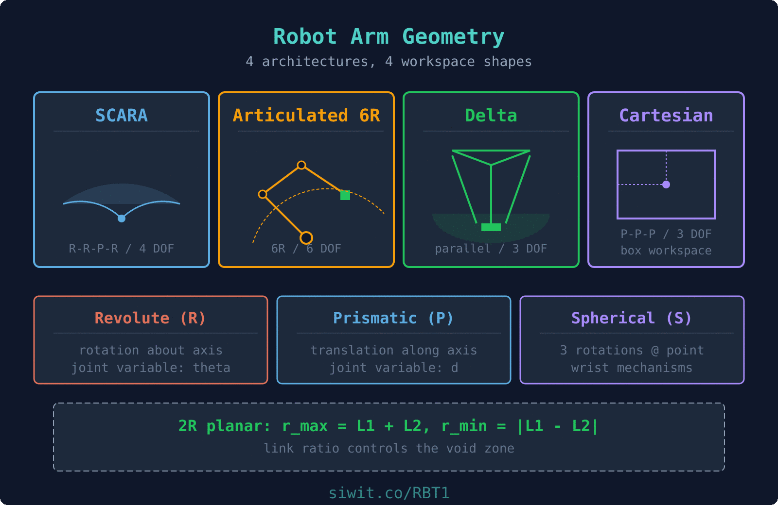
Compare common robot configurations: SCARA, articulated, delta, and Cartesian
Calculate reachable and dexterous workspace for a 2R planar arm
Visualize workspace boundaries using Python and matplotlib
Apply configuration selection criteria to real industrial pick-and-place problems

🔧 Real-World Engineering Challenge: Industrial Pick-and-Place Cell

A consumer electronics factory needs to automate the transfer of circuit boards between three stations: a solder reflow oven, an optical inspection camera, and a packaging tray. The boards arrive on a conveyor at a fixed height, pass through inspection at a raised platform, and must be placed into trays arranged in a grid pattern below. Cycle time is 4 seconds per board, and the cell footprint is limited to a 1.2 m by 1.2 m floor area. The engineering team must select a robot configuration that can reach all three stations within the space constraints while maintaining the required speed and precision.

Why This Problem Matters for Configuration Selection

Choosing the wrong robot configuration for a cell layout is one of the most expensive mistakes in automation. A 6-DOF articulated arm might seem like the safe choice for any task, but it could be slower, more expensive, and harder to program than a SCARA robot for this particular application. The geometry of the task, the shape of the required workspace, and the motion constraints all point toward specific configurations. Understanding arm geometry lets you make this selection with confidence before committing to hardware.

📚 Fundamental Theory: Robot Arm Structure

Links and Joints: The Building Blocks

A robot arm is a kinematic chain of rigid bodies called links, connected by joints that allow controlled relative motion between adjacent links. The first link is the base (fixed to the ground or a mounting surface), and the last link carries the end-effector (gripper, tool, or sensor). Every joint adds one or more degrees of freedom to the chain, and every link defines a geometric offset between the joints at its two ends.

Link Parameters

Each link in a robot arm is characterized by two geometric properties:

Link length (): the distance between adjacent joint axes, measured along the common normal
Link twist (): the angle between adjacent joint axes, measured about the common normal

These parameters, along with the joint variable, fully describe the relative position and orientation of consecutive links. We will formalize this using Denavit-Hartenberg parameters in a later lesson.

Joint Types

Joints constrain the relative motion between two links. The type of joint determines how many degrees of freedom it contributes and what kind of motion it allows.

Motion: Pure rotation about a single axis

DOF contributed: 1

Joint variable: Angle (radians or degrees)

Characteristics:

Most common joint type in industrial robots
Provides angular positioning
Compact design with high stiffness
Easily actuated by rotary motors

Workspace contribution: Each revolute joint sweeps an arc. Two revolute joints in series produce an annular (ring-shaped) workspace in the plane of rotation.

Degrees of Freedom

The total degrees of freedom of a robot arm determine how many independent motions it can perform simultaneously. For a serial chain (no closed loops), the total DOF is simply the sum of the DOF contributed by each joint. A task in 3D space requires up to 6 DOF for full positioning and orientation control: 3 for position (x, y, z) and 3 for orientation (roll, pitch, yaw).

For a serial manipulator with joints:

where is the number of degrees of freedom of joint .

Under-actuated (DOF < 6)

Cannot reach arbitrary positions and orientations in 3D space. Sufficient for tasks constrained to a plane or requiring only position control.

Examples: 2R planar arm (2 DOF), SCARA (4 DOF)

Fully-actuated (DOF = 6)

Can reach any reachable position with any feasible orientation. The minimum for general-purpose 3D manipulation.

Examples: Standard 6R industrial arms (KUKA, ABB, FANUC)

Redundant (DOF > 6)

More DOF than required for the task. Extra DOF provide flexibility for obstacle avoidance, singularity avoidance, or optimization of secondary criteria.

Examples: 7-DOF collaborative robots, dual-arm systems

Link Lengths and Their Effects

Link lengths directly control the size and shape of the robot’s workspace. Longer links increase reach but reduce stiffness and payload capacity. Shorter links improve rigidity and precision but limit the work volume. The ratio between link lengths in a serial chain also affects the shape of the reachable workspace and the distribution of dexterous regions within it.

For a planar 2R robot arm with link lengths and :

Maximum reach: (arm fully extended)
Minimum reach: (arm fully folded)
Workspace shape: Annular region between and

When , the inner radius goes to zero and the workspace becomes a full disk (the arm can reach the base). When , a “hole” appears at the center.

Workspace Analysis: Reachable vs. Dexterous

Workspace Definitions

Reachable workspace: The set of all points in space that the end-effector can reach with at least one orientation. This is the total volume the robot can access.
Dexterous workspace: The subset of the reachable workspace where the end-effector can achieve any arbitrary orientation. This is always smaller than or equal to the reachable workspace.
Void zone: Regions inside the reachable workspace boundary that the robot cannot access due to joint limits, self-collision, or mechanical interference.

Joint Limits and Their Impact

Real joints cannot rotate or translate indefinitely. Mechanical stops, cable routing, and safety considerations impose limits on every joint variable. These limits reduce the theoretical workspace to a smaller, sometimes oddly shaped, practical workspace. Joint limits also create configurations where the robot is near a boundary and has limited mobility in certain directions.

For a 2R arm with joint limits and :

If has a full 360° range, the workspace is rotationally symmetric
If is limited (e.g., 150°), the workspace becomes a sector of the annulus
If is limited, the inner and outer boundaries change shape

📐 Common Robot Configurations

Industrial robots come in several standard configurations, each designed for specific types of tasks. The configuration is defined by the sequence of joint types and the geometric arrangement of the links. Choosing the right configuration for a given application is one of the most important early decisions in robotic cell design.

SCARA (Selective Compliance Assembly Robot Arm)

Joint sequence: R-R-P-R (two revolute for planar motion, one prismatic for vertical, one revolute for end-effector rotation)

DOF: 4

Workspace shape: Cylindrical sector (fan-shaped in the horizontal plane, with vertical reach from the prismatic joint)

Key characteristics:

Very fast horizontal motion
Rigid in the vertical direction (good for insertion tasks)
Compliant in the horizontal plane (absorbs alignment errors)
Compact footprint

Typical applications:

PCB component insertion
Small parts assembly
Pick-and-place in electronics manufacturing
Screw driving

Workspace formula (horizontal plane):

with vertical stroke from the prismatic joint.

Configuration Comparison

Speed Champion: Delta

Accelerations up to 10g. Ideal when cycle time is the primary constraint and workspace volume is modest.

Versatility Champion: Articulated 6R

Full 6-DOF capability with large, flexible workspace. The default choice when task requirements are complex or varied.

Precision Assembly: SCARA

Fast horizontal motion with vertical rigidity. Purpose-built for insertion and assembly tasks in electronics.

Heavy Loads: Cartesian/Gantry

Highest stiffness and payload capacity. Best for large workspaces, heavy payloads, or applications where kinematic simplicity matters.

🖥️ Python Workspace Visualization

To build intuition about how link lengths and joint limits shape the workspace, let us compute and visualize the workspace of a planar 2R robot arm. The forward kinematics of a 2R arm maps joint angles to end-effector position, and by sweeping through all feasible joint angle combinations, we can trace the workspace boundary.

Forward Kinematics of a 2R Planar Arm

The end-effector position for a 2R arm with link lengths , and joint angles , :

Workspace Boundary Computation

import numpy as np
import matplotlib.pyplot as plt
from matplotlib.patches import Circle

def compute_2r_workspace(l1, l2, theta1_range, theta2_range, n_points=200):
    """
    Compute the workspace of a 2R planar robot arm.

    Parameters
    ----------
    l1 : float
        Length of link 1 (meters)
    l2 : float
        Length of link 2 (meters)
    theta1_range : tuple
        (min, max) angles for joint 1 in degrees
    theta2_range : tuple
        (min, max) angles for joint 2 in degrees
    n_points : int
        Number of sample points per joint

    Returns
    -------
    x, y : ndarray
        End-effector positions for all joint combinations
    """
    # Create joint angle grids
    theta1 = np.linspace(
        np.radians(theta1_range[0]),
        np.radians(theta1_range[1]),
        n_points
    )
    theta2 = np.linspace(
        np.radians(theta2_range[0]),
        np.radians(theta2_range[1]),
        n_points
    )

    # Meshgrid for all combinations
    T1, T2 = np.meshgrid(theta1, theta2)

    # Forward kinematics
    x = l1 * np.cos(T1) + l2 * np.cos(T1 + T2)
    y = l1 * np.sin(T1) + l2 * np.sin(T1 + T2)

    return x.flatten(), y.flatten()

def plot_workspace_comparison():
    """
    Compare workspaces for different link length ratios and joint limits.
    """
    fig, axes = plt.subplots(1, 3, figsize=(15, 5))

    # Configuration 1: Equal link lengths, full rotation
    x1, y1 = compute_2r_workspace(
        l1=0.4, l2=0.4,
        theta1_range=(0, 360),
        theta2_range=(0, 360)
    )
    axes[0].scatter(x1, y1, s=0.1, alpha=0.3, c='steelblue')
    axes[0].set_title('Equal links (0.4, 0.4)\nFull rotation')
    axes[0].set_aspect('equal')
    axes[0].set_xlabel('x (m)')
    axes[0].set_ylabel('y (m)')
    axes[0].grid(True, alpha=0.3)
    # Mark the origin (base)
    axes[0].plot(0, 0, 'ko', markersize=8)

    # Configuration 2: Unequal link lengths, full rotation
    x2, y2 = compute_2r_workspace(
        l1=0.5, l2=0.3,
        theta1_range=(0, 360),
        theta2_range=(0, 360)
    )
    axes[1].scatter(x2, y2, s=0.1, alpha=0.3, c='coral')
    axes[1].set_title('Unequal links (0.5, 0.3)\nFull rotation')
    axes[1].set_aspect('equal')
    axes[1].set_xlabel('x (m)')
    axes[1].set_ylabel('y (m)')
    axes[1].grid(True, alpha=0.3)
    axes[1].plot(0, 0, 'ko', markersize=8)
    # Show the inner void
    void_circle = Circle((0, 0), 0.2, fill=False,
                          linestyle='--', color='red', linewidth=1.5)
    axes[1].add_patch(void_circle)
    axes[1].annotate('Void zone\nr = |l1 - l2|', xy=(0.14, 0.14),
                     fontsize=8, color='red')

    # Configuration 3: Equal links, limited joints
    x3, y3 = compute_2r_workspace(
        l1=0.4, l2=0.4,
        theta1_range=(-150, 150),
        theta2_range=(-135, 135)
    )
    axes[2].scatter(x3, y3, s=0.1, alpha=0.3, c='forestgreen')
    axes[2].set_title('Equal links (0.4, 0.4)\nLimited joints')
    axes[2].set_aspect('equal')
    axes[2].set_xlabel('x (m)')
    axes[2].set_ylabel('y (m)')
    axes[2].grid(True, alpha=0.3)
    axes[2].plot(0, 0, 'ko', markersize=8)

    plt.tight_layout()
    plt.savefig('2r_workspace_comparison.png', dpi=150, bbox_inches='tight')
    plt.show()

# Run the visualization
plot_workspace_comparison()

Visualizing a Single Arm Configuration

import numpy as np
import matplotlib.pyplot as plt

def draw_2r_arm(l1, l2, theta1_deg, theta2_deg, ax, color='steelblue'):
    """
    Draw a 2R planar arm at a specific configuration.

    Parameters
    ----------
    l1, l2 : float
        Link lengths
    theta1_deg, theta2_deg : float
        Joint angles in degrees
    ax : matplotlib axis
        Axis to draw on
    color : str
        Color for the arm links
    """
    theta1 = np.radians(theta1_deg)
    theta2 = np.radians(theta2_deg)

    # Joint positions
    base = np.array([0, 0])
    elbow = np.array([l1 * np.cos(theta1),
                      l1 * np.sin(theta1)])
    end_effector = np.array([
        l1 * np.cos(theta1) + l2 * np.cos(theta1 + theta2),
        l1 * np.sin(theta1) + l2 * np.sin(theta1 + theta2)
    ])

    # Draw links
    ax.plot([base[0], elbow[0]], [base[1], elbow[1]],
            '-o', color=color, linewidth=3, markersize=8,
            markerfacecolor='white', markeredgecolor=color,
            markeredgewidth=2)
    ax.plot([elbow[0], end_effector[0]], [elbow[1], end_effector[1]],
            '-o', color=color, linewidth=3, markersize=8,
            markerfacecolor='white', markeredgecolor=color,
            markeredgewidth=2)

    # Mark end-effector
    ax.plot(end_effector[0], end_effector[1], 's',
            color='red', markersize=10)

    # Mark base
    ax.plot(base[0], base[1], 'ko', markersize=12)

    return end_effector

def show_multiple_configurations():
    """
    Show the same 2R arm in several configurations to illustrate
    how joint angles map to end-effector positions.
    """
    fig, ax = plt.subplots(1, 1, figsize=(8, 8))

    l1, l2 = 0.4, 0.35

    # Draw workspace background
    x_ws, y_ws = compute_2r_workspace(
        l1, l2,
        theta1_range=(0, 360),
        theta2_range=(0, 360),
        n_points=300
    )
    ax.scatter(x_ws, y_ws, s=0.05, alpha=0.1, c='lightgray')

    # Draw arm in several configurations
    configs = [
        (30, 45, 'steelblue'),
        (90, -60, 'coral'),
        (150, 90, 'forestgreen'),
        (210, -30, 'purple'),
        (-45, 120, 'orange'),
    ]

    for theta1, theta2, color in configs:
        end = draw_2r_arm(l1, l2, theta1, theta2, ax, color=color)
        ax.annotate(
            f'({theta1}\u00b0, {theta2}\u00b0)',
            xy=end, fontsize=7,
            textcoords="offset points", xytext=(8, 8)
        )

    ax.set_xlim(-0.9, 0.9)
    ax.set_ylim(-0.9, 0.9)
    ax.set_aspect('equal')
    ax.set_xlabel('x (m)')
    ax.set_ylabel('y (m)')
    ax.set_title('2R Arm: Multiple Configurations in Workspace')
    ax.grid(True, alpha=0.3)

    plt.tight_layout()
    plt.savefig('2r_arm_configurations.png', dpi=150, bbox_inches='tight')
    plt.show()

show_multiple_configurations()

Comparing Robot Configurations

import numpy as np
import matplotlib.pyplot as plt

def scara_workspace_topview(l1, l2, theta1_range, theta2_range, n=200):
    """
    Compute the top-view (XY plane) workspace of a SCARA robot.
    Same as 2R workspace since SCARA horizontal motion is 2R.
    """
    return compute_2r_workspace(l1, l2, theta1_range, theta2_range, n)

def cartesian_workspace_topview(x_range, y_range, n=200):
    """
    Compute the top-view workspace of a Cartesian robot.
    Simply a rectangle.
    """
    x = np.linspace(x_range[0], x_range[1], n)
    y = np.linspace(y_range[0], y_range[1], n)
    X, Y = np.meshgrid(x, y)
    return X.flatten(), Y.flatten()

def delta_workspace_topview(r_base, r_ee, l_upper, l_lower, n=300):
    """
    Approximate top-view workspace of a delta robot.
    The workspace is roughly a circle centered below the base.

    Parameters
    ----------
    r_base : float
        Radius of the base platform
    r_ee : float
        Radius of the end-effector platform
    l_upper : float
        Length of upper arms
    l_lower : float
        Length of lower arms (parallelogram linkages)
    n : int
        Number of sample angles
    """
    # Approximate effective horizontal reach
    r_max = l_lower * 0.7  # empirical factor for typical delta geometry
    theta = np.linspace(0, 2 * np.pi, n)
    radii = np.linspace(0, r_max, n // 2)
    T, R = np.meshgrid(theta, radii)
    x = R.flatten() * np.cos(T.flatten())
    y = R.flatten() * np.sin(T.flatten())
    return x, y

def compare_configurations():
    """
    Side-by-side comparison of workspace shapes for four robot types.
    """
    fig, axes = plt.subplots(2, 2, figsize=(12, 12))

    # SCARA (top view)
    x, y = scara_workspace_topview(
        l1=0.35, l2=0.30,
        theta1_range=(-135, 135),
        theta2_range=(-150, 150)
    )
    axes[0, 0].scatter(x, y, s=0.2, alpha=0.3, c='steelblue')
    axes[0, 0].set_title('SCARA (Top View)', fontsize=12, fontweight='bold')
    axes[0, 0].set_xlabel('x (m)')
    axes[0, 0].set_ylabel('y (m)')
    axes[0, 0].set_aspect('equal')
    axes[0, 0].grid(True, alpha=0.3)
    axes[0, 0].plot(0, 0, 'ko', markersize=8)

    # Articulated 6R (simplified top view, similar to SCARA
    # but with larger angular range)
    x, y = scara_workspace_topview(
        l1=0.40, l2=0.35,
        theta1_range=(-170, 170),
        theta2_range=(-160, 160)
    )
    axes[0, 1].scatter(x, y, s=0.2, alpha=0.3, c='coral')
    axes[0, 1].set_title('Articulated 6R (Top View)', fontsize=12,
                          fontweight='bold')
    axes[0, 1].set_xlabel('x (m)')
    axes[0, 1].set_ylabel('y (m)')
    axes[0, 1].set_aspect('equal')
    axes[0, 1].grid(True, alpha=0.3)
    axes[0, 1].plot(0, 0, 'ko', markersize=8)

    # Delta (top view)
    x, y = delta_workspace_topview(
        r_base=0.15, r_ee=0.05,
        l_upper=0.20, l_lower=0.40
    )
    axes[1, 0].scatter(x, y, s=0.2, alpha=0.3, c='forestgreen')
    axes[1, 0].set_title('Delta (Top View)', fontsize=12, fontweight='bold')
    axes[1, 0].set_xlabel('x (m)')
    axes[1, 0].set_ylabel('y (m)')
    axes[1, 0].set_aspect('equal')
    axes[1, 0].grid(True, alpha=0.3)
    axes[1, 0].plot(0, 0, 'ko', markersize=8)

    # Cartesian (top view)
    x, y = cartesian_workspace_topview(
        x_range=(-0.4, 0.4),
        y_range=(-0.3, 0.3)
    )
    axes[1, 1].scatter(x, y, s=0.2, alpha=0.3, c='purple')
    axes[1, 1].set_title('Cartesian (Top View)', fontsize=12,
                          fontweight='bold')
    axes[1, 1].set_xlabel('x (m)')
    axes[1, 1].set_ylabel('y (m)')
    axes[1, 1].set_aspect('equal')
    axes[1, 1].grid(True, alpha=0.3)

    plt.suptitle('Workspace Shape Comparison (Top View)',
                 fontsize=14, fontweight='bold', y=1.01)
    plt.tight_layout()
    plt.savefig('robot_workspace_comparison.png', dpi=150,
                bbox_inches='tight')
    plt.show()

compare_configurations()

🎯 System Application: Solving the Pick-and-Place Problem

Let us return to the circuit board handling cell and apply what we have learned about arm geometry and configuration selection. The three stations (reflow oven output, inspection camera, packaging tray) define the workspace requirements, and the footprint constraint limits our configuration choices.

Station Layout Analysis

Map the station positions

Place the robot base at the center of the 1.2 m x 1.2 m cell. The three stations are located at approximately:
- Conveyor pickup: (0.45, 0.15) m from base
- Inspection camera: (0.10, 0.50) m from base (raised platform)
- Packaging tray grid: (-0.30, 0.35) m from base (below base height)
All three points must lie within the robot’s reachable workspace.
Calculate required reach

Maximum distance from base to any station:

The inspection station is the farthest point, requiring at least 0.51 m reach.
Determine DOF requirements

The task involves:
- Horizontal positioning (2 DOF)
- Vertical motion to pick up and place boards (1 DOF)
- Rotation to align board orientation (1 DOF)
Total: 4 DOF minimum. No arbitrary 3D orientation is needed.
Select configuration

With 4 DOF, horizontal planar motion, vertical pick-and-place, and a compact footprint requirement, the SCARA configuration is the clear choice.

SCARA Sizing for the Cell

Link length selection and workspace verification

For a SCARA with links and :

Selected dimensions:

m, m
m (covers all stations with margin)
m (small void zone near the base)
Vertical stroke: 150 mm (sufficient for conveyor-to-tray height difference)

Verification:

Conveyor (0.47 m): within reach (0.47 < 0.55)
Inspection (0.51 m): within reach (0.51 < 0.55)
Tray (0.46 m): within reach (0.46 < 0.55)
All stations outside void zone (all > 0.05 m)

Why Not Other Configurations?

Articulated 6R

Overkill for this task. 6 DOF when only 4 are needed. Higher cost, more complex programming, slower for simple horizontal pick-and-place motions.

Delta

Excellent speed, but limited workspace volume. With a 1.2 m cell and stations spread at 0.5 m from center, a delta robot would need very long arms, reducing its speed advantage.

Cartesian

Could work, but the gantry structure would take significant overhead space. Also slower than SCARA for the cycle time requirement of 4 seconds per board.

🛠️ Design Guidelines

Configuration Selection Rules

Start with the task DOF

Count the independent motions the end-effector must perform. If only planar positioning is needed, 3 DOF suffices. If full 3D positioning and orientation are needed, 6 DOF is the minimum.
Match workspace shape to station layout

SCARA and articulated arms produce annular workspaces. Cartesian robots produce rectangular workspaces. Delta robots produce dome-shaped volumes. Choose the shape that covers your stations most efficiently.
Size links using the reach equation

For serial arms: (all links extended). Ensure exceeds the farthest station distance by at least 10% for margin.
Check the void zone

For 2R and SCARA: . Ensure no stations lie within this radius. If they do, adjust link ratios.
Verify joint limits do not exclude stations

Plot the actual workspace with joint limits applied. Confirm all stations and the paths between them lie within the feasible region.
Consider cycle time and payload

Faster configurations (delta, SCARA) trade workspace volume for speed. Heavier payloads favor Cartesian or articulated designs with higher stiffness.

Common Design Pitfalls

📋 Summary

This lesson covered the structural foundations of robot arm design:

Links and joints form the building blocks. Revolute joints provide rotation, prismatic joints provide translation, and the combination defines the arm’s motion capability.
Link lengths determine reach. For a 2R arm, and . The link ratio controls the void zone size.
Joint limits reduce the theoretical workspace to a practical workspace. Always design with real joint limits, not ideal full-rotation assumptions.
Four standard configurations cover most industrial applications: SCARA for fast planar assembly, articulated 6R for general-purpose manipulation, delta for high-speed pick-and-place, and Cartesian for large rectangular workspaces.
Configuration selection should be driven by task DOF, workspace shape, station layout, cycle time, and payload requirements.

Coming Next: In Lesson 2, we will formalize the relationship between joint angles and end-effector position using forward kinematics and the Denavit-Hartenberg convention, building the mathematical framework for precise robot motion control.

Comments

Loading comments...