Lattice Structures & TPMS for Additive Manufacturing

Modified: Mar. 4, 2026

Published: Mar. 4, 2026

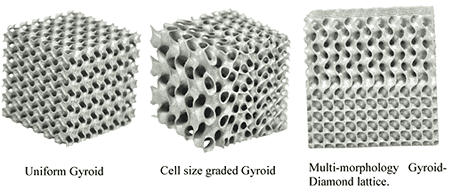
Create lightweight lattice structures and triply periodic minimal surfaces (TPMS) that are impossible to model by hand in traditional CAD. Using CadQuery and NumPy, you will generate strut-based unit cells, implicit gyroid and Schwarz-P surfaces, graded-density fills, and conformal lattices ready for SLA, SLS, or FDM printing. #LatticeDesign #TPMS #AdditiveManufacturing

Learning Objectives

By the end of this lesson, you will be able to:

Generate strut-based unit cells (cubic, BCC, octet-truss) and array them into lattice volumes
Implement TPMS implicit surfaces using trigonometric equations (gyroid, Schwarz-P, diamond)
Control graded density by varying strut thickness or TPMS threshold across a volume
Apply conformal lattice filling to arbitrary 3D shapes
Evaluate printability constraints for SLA, SLS, and FDM processes

Why Lattice Structures?

Weight Reduction

Lattice-filled parts can achieve 50-90% weight reduction compared to solid equivalents while retaining a significant fraction of structural stiffness and strength.

Energy Absorption

Controlled cell collapse provides predictable energy absorption profiles, critical for crash structures, protective equipment, and packaging.

Biomedical Integration

Porous lattices match the stiffness of bone (reducing stress shielding) and promote osseointegration in orthopedic implants.

Thermal Management

High surface-area-to-volume ratios in TPMS structures create excellent heat exchanger geometries with low pressure drop.

Strut-Based Lattice Fundamentals

Strut-based lattices are constructed from wireframe unit cells: nodes connected by cylindrical or tapered struts. The unit cell is then arrayed in three dimensions to fill a volume.

Unit Cell Geometry

The three most common strut-based unit cells differ in their connectivity, which directly determines mechanical properties:

Unit Cell	Nodes	Struts	Connectivity	Relative Density Range
Simple Cubic (SC)	8	12	Edge-connected	5-30%
Body-Centered Cubic (BCC)	9	8	Diagonal body struts	5-40%
Octet-Truss	14	36	Face + body diagonals	10-50%

The relative density is the ratio of lattice density to the density of the solid material:

For cylindrical struts of diameter in a cubic cell of side length , the relative density of a BCC lattice is approximately:

CadQuery Strut-Based Lattice Implementation

The simple cubic unit cell connects the eight corner nodes with struts along the twelve edges.

import cadquery as cq
import numpy as np

def cubic_unit_cell(cell_size: float, strut_diameter: float) -> cq.Workplane:
    """Generate a simple cubic unit cell.

    Args:
        cell_size: Edge length of the cubic cell (mm)
        strut_diameter: Diameter of cylindrical struts (mm)

    Returns:
        CadQuery solid of one unit cell
    """
    L = cell_size
    r = strut_diameter / 2.0
    result = cq.Workplane("XY")

    # Define the 12 edges of a cube as (start, end) coordinate pairs
    edges = [
        # Bottom face edges
        ((0, 0, 0), (L, 0, 0)),
        ((L, 0, 0), (L, L, 0)),
        ((L, L, 0), (0, L, 0)),
        ((0, L, 0), (0, 0, 0)),
        # Top face edges
        ((0, 0, L), (L, 0, L)),
        ((L, 0, L), (L, L, L)),
        ((L, L, L), (0, L, L)),
        ((0, L, L), (0, 0, L)),
        # Vertical edges
        ((0, 0, 0), (0, 0, L)),
        ((L, 0, 0), (L, 0, L)),
        ((L, L, 0), (L, L, L)),
        ((0, L, 0), (0, L, L)),
    ]

    # Build each strut as a cylinder between two points
    struts = []
    for (x1, y1, z1), (x2, y2, z2) in edges:
        mid_x = (x1 + x2) / 2
        mid_y = (y1 + y2) / 2
        mid_z = (z1 + z2) / 2
        length = np.sqrt((x2-x1)**2 + (y2-y1)**2 + (z2-z1)**2)

        # Determine strut direction for orientation
        dx, dy, dz = x2 - x1, y2 - y1, z2 - z1

        strut = (
            cq.Workplane("XY")
            .transformed(offset=(mid_x, mid_y, mid_z))
            .cylinder(length, r, centered=(True, True, True))
        )
        struts.append(strut)

    # Union all struts together
    result = struts[0]
    for s in struts[1:]:
        result = result.union(s)

    # Add spherical nodes at corners for smooth joints
    for x in [0, L]:
        for y in [0, L]:
            for z in [0, L]:
                node = cq.Workplane("XY").newObject([
                    cq.Solid.makeSphere(r * 1.2, pnt=cq.Vector(x, y, z))
                ])
                result = result.union(node)

    return result

# Generate a 10mm cubic cell with 1mm struts
cell = cubic_unit_cell(cell_size=10.0, strut_diameter=1.0)

The BCC unit cell connects each corner node to the center node, producing eight diagonal struts.

import cadquery as cq
import numpy as np
from typing import Tuple

def make_strut(p1: Tuple[float, float, float],
               p2: Tuple[float, float, float],
               diameter: float) -> cq.Workplane:
    """Create a cylindrical strut between two 3D points.

    Uses the wire-and-sweep approach for arbitrary orientations.
    """
    wire = cq.Workplane("XY").moveTo(p1[0], p1[1]).lineTo(p2[0], p2[1])
    # For true 3D struts, use the polyline + sweep approach
    path = (
        cq.Workplane("XY")
        .pushPoints([p1])
        .workplane()
        .moveTo(0, 0)
        .threePointArc((0, 0, 0), (0, 0, 0))  # placeholder
    )

    # Simpler approach: calculate midpoint, length, and orientation
    mid = tuple((a + b) / 2 for a, b in zip(p1, p2))
    length = np.sqrt(sum((b - a)**2 for a, b in zip(p1, p2)))
    direction = tuple((b - a) / length for a, b in zip(p1, p2))

    # Create cylinder along Z, then rotate to align with direction
    r = diameter / 2.0
    strut = cq.Workplane("XY").cylinder(length, r)

    # Compute rotation to align Z-axis with strut direction
    z_axis = np.array([0, 0, 1])
    d = np.array(direction)

    if np.allclose(d, z_axis):
        rotation_axis = (0, 0, 1)
        angle = 0
    elif np.allclose(d, -z_axis):
        rotation_axis = (1, 0, 0)
        angle = 180
    else:
        rot_ax = np.cross(z_axis, d)
        rot_ax = rot_ax / np.linalg.norm(rot_ax)
        angle = np.degrees(np.arccos(np.clip(np.dot(z_axis, d), -1, 1)))
        rotation_axis = tuple(rot_ax)

    strut = strut.val().Rotate(
        (0, 0, 0), rotation_axis, angle
    )
    strut = cq.Workplane("XY").add(strut).translate(mid)

    return strut

def bcc_unit_cell(cell_size: float, strut_diameter: float) -> cq.Workplane:
    """Generate a BCC unit cell.

    Eight diagonal struts connect corners to body center.
    """
    L = cell_size
    r = strut_diameter / 2.0
    center = (L/2, L/2, L/2)

    # BCC: 8 corners connected to body center
    corners = [
        (0, 0, 0), (L, 0, 0), (L, L, 0), (0, L, 0),
        (0, 0, L), (L, 0, L), (L, L, L), (0, L, L),
    ]

    struts = []
    for corner in corners:
        strut = make_strut(corner, center, strut_diameter)
        struts.append(strut)

    # Union all struts
    result = struts[0]
    for s in struts[1:]:
        result = result.union(s)

    # Add spherical nodes
    all_nodes = corners + [center]
    for node_pos in all_nodes:
        node = cq.Workplane("XY").newObject([
            cq.Solid.makeSphere(r * 1.3, pnt=cq.Vector(*node_pos))
        ])
        result = result.union(node)

    return result

# Generate a BCC cell: 10mm size, 0.8mm struts
bcc_cell = bcc_unit_cell(cell_size=10.0, strut_diameter=0.8)

The octet-truss is the highest-performance strut lattice. It combines face-centered and body-centered connectivity to create a stretch-dominated structure (much stiffer than bending-dominated alternatives at the same relative density).

import cadquery as cq
import numpy as np

def octet_truss_unit_cell(cell_size: float,
                          strut_diameter: float) -> cq.Workplane:
    """Generate an octet-truss unit cell.

    14 nodes: 8 corners + 6 face centers
    36 struts connecting nearest neighbors
    """
    L = cell_size
    r = strut_diameter / 2.0

    # 8 corner nodes
    corners = [
        (0, 0, 0), (L, 0, 0), (L, L, 0), (0, L, 0),
        (0, 0, L), (L, 0, L), (L, L, L), (0, L, L),
    ]

    # 6 face center nodes
    face_centers = [
        (L/2, L/2, 0),   # bottom
        (L/2, L/2, L),   # top
        (L/2, 0, L/2),   # front
        (L/2, L, L/2),   # back
        (0, L/2, L/2),   # left
        (L, L/2, L/2),   # right
    ]

    all_nodes = corners + face_centers

    # Connect each face center to the 4 corners of its face
    # Plus connect face centers to each other through body diagonals
    connections = []

    # Bottom face center (index 8) to bottom corners
    connections += [(8, 0), (8, 1), (8, 2), (8, 3)]
    # Top face center (index 9) to top corners
    connections += [(9, 4), (9, 5), (9, 6), (9, 7)]
    # Front face center (index 10) to front corners
    connections += [(10, 0), (10, 1), (10, 4), (10, 5)]
    # Back face center (index 11) to back corners
    connections += [(11, 2), (11, 3), (11, 6), (11, 7)]
    # Left face center (index 12) to left corners
    connections += [(12, 0), (12, 3), (12, 4), (12, 7)]
    # Right face center (index 13) to right corners
    connections += [(13, 1), (13, 2), (13, 5), (13, 6)]

    # Cross-connections between face centers (internal bracing)
    connections += [
        (8, 9), (8, 10), (8, 11), (8, 12), (8, 13),
        (9, 10), (9, 11), (9, 12), (9, 13),
        (10, 11), (10, 12), (10, 13),
        (11, 12), (11, 13),
        (12, 13),
    ]

    struts = []
    for i, j in connections:
        p1 = all_nodes[i]
        p2 = all_nodes[j]
        strut = make_strut(p1, p2, strut_diameter)
        struts.append(strut)

    # Union all struts
    result = struts[0]
    for s in struts[1:]:
        result = result.union(s)

    # Spherical joints at all nodes
    for pos in all_nodes:
        node = cq.Workplane("XY").newObject([
            cq.Solid.makeSphere(r * 1.4, pnt=cq.Vector(*pos))
        ])
        result = result.union(node)

    return result

# Octet-truss: 12mm cell, 0.6mm struts
octet = octet_truss_unit_cell(cell_size=12.0, strut_diameter=0.6)

Arraying Unit Cells into a Lattice Volume

Once a unit cell is defined, you array it by translating copies across a 3D grid:

def array_lattice(unit_cell_func, cell_size: float,
                  strut_diameter: float,
                  nx: int, ny: int, nz: int) -> cq.Assembly:
    """Array a unit cell into an nx × ny × nz lattice block.

    Args:
        unit_cell_func: Function that returns a unit cell solid
        cell_size: Size of each unit cell (mm)
        strut_diameter: Strut diameter (mm)
        nx, ny, nz: Number of cells in each direction

    Returns:
        CadQuery Assembly of arrayed cells
    """
    assembly = cq.Assembly()

    # Generate one cell and reuse it
    cell = unit_cell_func(cell_size, strut_diameter)

    for ix in range(nx):
        for iy in range(ny):
            for iz in range(nz):
                offset = (
                    ix * cell_size,
                    iy * cell_size,
                    iz * cell_size,
                )
                assembly.add(
                    cell,
                    loc=cq.Location(cq.Vector(*offset)),
                    name=f"cell_{ix}_{iy}_{iz}",
                )

    return assembly

# Create a 4x4x4 BCC lattice block
lattice_block = array_lattice(
    bcc_unit_cell,
    cell_size=8.0,
    strut_diameter=0.8,
    nx=4, ny=4, nz=4
)

Triply Periodic Minimal Surfaces (TPMS)

TPMS are mathematically-defined surfaces that are periodic in all three spatial directions and have zero mean curvature at every point. They produce smooth, self-supporting geometries that are often superior to strut-based lattices for load-bearing and fluid-flow applications.

TPMS Implicit Surface Equations

A TPMS is defined by an implicit equation , where is the threshold (or level-set value) that controls the wall thickness and relative density. The three most common TPMS types are:

The gyroid is the most widely used TPMS in engineering. It has no straight lines, no planar symmetries, and is completely self-supporting (no overhangs greater than ~45 degrees).

where is the unit cell period and controls the volume fraction. At , the surface divides space into two equal, interpenetrating volumes.

Key property: The gyroid is self-supporting for most AM processes because maximum overhang angles stay below 42 degrees.

Relationship Between Threshold and Relative Density

The threshold parameter directly controls the relative density :

TPMS Type	(Relative Density)
Gyroid	~50%	~35%	~20%
Schwarz-P	~50%	~30%	~15%
Diamond	~50%	~33%	~18%

TPMS Implementation with CadQuery and NumPy

Generating TPMS geometry involves evaluating the implicit function on a 3D voxel grid, then extracting an isosurface using the marching cubes algorithm. The resulting triangle mesh is converted into a CadQuery solid.

Step 1: Evaluate the Implicit Function

import numpy as np
from scipy import ndimage

def evaluate_tpms(tpms_type: str,
                  bounds: tuple,
                  resolution: int,
                  period: float,
                  threshold: float = 0.0) -> np.ndarray:
    """Evaluate a TPMS implicit function on a 3D grid.

    Args:
        tpms_type: One of 'gyroid', 'schwarz_p', 'diamond'
        bounds: (xmin, xmax, ymin, ymax, zmin, zmax) in mm
        resolution: Number of voxels per axis
        period: Unit cell period L (mm)
        threshold: Level-set value t

    Returns:
        3D numpy array of function values
    """
    xmin, xmax, ymin, ymax, zmin, zmax = bounds
    x = np.linspace(xmin, xmax, resolution)
    y = np.linspace(ymin, ymax, resolution)
    z = np.linspace(zmin, zmax, resolution)
    X, Y, Z = np.meshgrid(x, y, z, indexing='ij')

    # Scale to unit cell period
    kx = 2 * np.pi * X / period
    ky = 2 * np.pi * Y / period
    kz = 2 * np.pi * Z / period

    if tpms_type == 'gyroid':
        F = (np.sin(kx) * np.cos(ky) +
             np.sin(ky) * np.cos(kz) +
             np.sin(kz) * np.cos(kx))
    elif tpms_type == 'schwarz_p':
        F = np.cos(kx) + np.cos(ky) + np.cos(kz)
    elif tpms_type == 'diamond':
        F = (np.cos(kx) * np.cos(ky) * np.cos(kz) -
             np.sin(kx) * np.sin(ky) * np.sin(kz))
    else:
        raise ValueError(f"Unknown TPMS type: {tpms_type}")

    # Return binary volume: 1 where F > threshold, 0 elsewhere
    return (F - threshold)

# Example: Gyroid in a 40mm cube, 10mm period
field = evaluate_tpms(
    'gyroid',
    bounds=(0, 40, 0, 40, 0, 40),
    resolution=100,
    period=10.0,
    threshold=0.0
)

Step 2: Extract Isosurface with Marching Cubes

from skimage.measure import marching_cubes
import trimesh

def field_to_mesh(field: np.ndarray,
                  bounds: tuple,
                  level: float = 0.0) -> trimesh.Trimesh:
    """Convert a 3D scalar field to a triangle mesh.

    Args:
        field: 3D numpy array from evaluate_tpms
        bounds: Physical bounds (xmin, xmax, ymin, ymax, zmin, zmax)
        level: Isosurface level (usually 0.0)

    Returns:
        trimesh.Trimesh object
    """
    xmin, xmax, ymin, ymax, zmin, zmax = bounds
    spacing = (
        (xmax - xmin) / (field.shape[0] - 1),
        (ymax - ymin) / (field.shape[1] - 1),
        (zmax - zmin) / (field.shape[2] - 1),
    )

    verts, faces, normals, _ = marching_cubes(
        field, level=level, spacing=spacing
    )

    # Offset vertices to match physical bounds
    verts[:, 0] += xmin
    verts[:, 1] += ymin
    verts[:, 2] += zmin

    mesh = trimesh.Trimesh(
        vertices=verts, faces=faces, vertex_normals=normals
    )

    return mesh

# Extract the isosurface
mesh = field_to_mesh(field, bounds=(0, 40, 0, 40, 0, 40))
mesh.export("gyroid_40mm.stl")
print(f"Mesh: {len(mesh.vertices)} vertices, {len(mesh.faces)} faces")

Step 3: Convert Mesh to CadQuery Solid (Optional)

For boolean operations with CadQuery shapes, you can import the STL back as a solid:

import cadquery as cq

def stl_to_cadquery(stl_path: str) -> cq.Workplane:
    """Import an STL file as a CadQuery solid.

    Note: This requires the STL to be a valid, watertight mesh.
    """
    result = cq.importers.importStl(stl_path)
    return cq.Workplane("XY").add(result)

# Import gyroid mesh as CadQuery solid
gyroid_solid = stl_to_cadquery("gyroid_40mm.stl")

Sheet TPMS Generation

To create a thin-walled sheet TPMS (higher specific stiffness than solid TPMS):

def sheet_tpms(tpms_type: str, bounds: tuple, resolution: int,
               period: float, wall_thickness: float) -> trimesh.Trimesh:
    """Generate a sheet TPMS with defined wall thickness.

    Creates geometry where: -t/2 < f(x,y,z) < t/2

    Args:
        wall_thickness: Desired wall thickness in mm
        (other args as in evaluate_tpms)
    """
    field = evaluate_tpms(tpms_type, bounds, resolution, period,
                          threshold=0.0)

    # The threshold range maps approximately to wall thickness
    # Calibration: for gyroid with period L, threshold range dt
    # gives wall_thickness ≈ dt * L / (2*pi)
    dt = wall_thickness * 2 * np.pi / period

    # Sheet region: |f(x,y,z)| < dt/2
    sheet_field = np.abs(field) - dt / 2

    # Extract outer surface (where sheet_field = 0)
    mesh = field_to_mesh(-sheet_field, bounds)

    return mesh

# 0.4mm wall sheet gyroid
sheet = sheet_tpms(
    'gyroid',
    bounds=(0, 30, 0, 30, 0, 30),
    resolution=150,
    period=8.0,
    wall_thickness=0.4
)
sheet.export("gyroid_sheet_30mm.stl")

Graded Density Lattices

Uniform lattices have the same density everywhere, but real load paths are not uniform. Graded lattices vary the density spatially, placing more material where stresses are high and less where loads are low.

Approach 1: Graded Strut Thickness

For strut-based lattices, vary the strut diameter as a function of position:

def graded_bcc_lattice(cell_size: float,
                       nx: int, ny: int, nz: int,
                       d_min: float, d_max: float,
                       gradient_axis: str = 'z') -> cq.Assembly:
    """Generate a BCC lattice with linearly graded strut diameter.

    Args:
        cell_size: Unit cell size (mm)
        nx, ny, nz: Number of cells per axis
        d_min: Minimum strut diameter (mm) at gradient start
        d_max: Maximum strut diameter (mm) at gradient end
        gradient_axis: Axis along which density varies ('x', 'y', 'z')
    """
    assembly = cq.Assembly()

    # Map axis to cell count
    n_gradient = {'x': nx, 'y': ny, 'z': nz}[gradient_axis]

    for ix in range(nx):
        for iy in range(ny):
            for iz in range(nz):
                # Compute gradient parameter (0 to 1)
                if gradient_axis == 'z':
                    t = iz / max(nz - 1, 1)
                elif gradient_axis == 'y':
                    t = iy / max(ny - 1, 1)
                else:
                    t = ix / max(nx - 1, 1)

                # Linear interpolation of strut diameter
                d = d_min + t * (d_max - d_min)

                cell = bcc_unit_cell(cell_size, d)
                offset = (
                    ix * cell_size,
                    iy * cell_size,
                    iz * cell_size
                )
                assembly.add(
                    cell,
                    loc=cq.Location(cq.Vector(*offset)),
                    name=f"cell_{ix}_{iy}_{iz}_d{d:.2f}",
                )

    return assembly

# Graded BCC: thin at bottom (0.4mm), thick at top (1.2mm)
graded = graded_bcc_lattice(
    cell_size=8.0,
    nx=5, ny=5, nz=8,
    d_min=0.4, d_max=1.2,
    gradient_axis='z'
)

Approach 2: Graded TPMS Threshold

For TPMS, spatially vary the threshold parameter :

where is no longer constant but a function of position:

def graded_tpms(tpms_type: str, bounds: tuple, resolution: int,
                period: float, t_min: float, t_max: float,
                gradient_axis: str = 'z') -> np.ndarray:
    """Evaluate TPMS with spatially varying threshold.

    Creates a density gradient: dense where t is small,
    sparse where t is large.
    """
    xmin, xmax, ymin, ymax, zmin, zmax = bounds
    x = np.linspace(xmin, xmax, resolution)
    y = np.linspace(ymin, ymax, resolution)
    z = np.linspace(zmin, zmax, resolution)
    X, Y, Z = np.meshgrid(x, y, z, indexing='ij')

    # Compute TPMS field
    kx = 2 * np.pi * X / period
    ky = 2 * np.pi * Y / period
    kz = 2 * np.pi * Z / period

    if tpms_type == 'gyroid':
        F = (np.sin(kx) * np.cos(ky) +
             np.sin(ky) * np.cos(kz) +
             np.sin(kz) * np.cos(kx))
    elif tpms_type == 'schwarz_p':
        F = np.cos(kx) + np.cos(ky) + np.cos(kz)
    else:
        raise ValueError(f"Unknown type: {tpms_type}")

    # Spatially varying threshold
    if gradient_axis == 'z':
        # Normalize Z to [0, 1] range
        T = t_min + (t_max - t_min) * (Z - zmin) / (zmax - zmin)
    elif gradient_axis == 'y':
        T = t_min + (t_max - t_min) * (Y - ymin) / (ymax - ymin)
    else:
        T = t_min + (t_max - t_min) * (X - xmin) / (xmax - xmin)

    return F - T

# Dense at bottom (t=0.0), sparse at top (t=0.8)
graded_field = graded_tpms(
    'gyroid',
    bounds=(0, 40, 0, 40, 0, 60),
    resolution=120,
    period=8.0,
    t_min=0.0, t_max=0.8,
    gradient_axis='z'
)

graded_mesh = field_to_mesh(graded_field, (0, 40, 0, 40, 0, 60))
graded_mesh.export("gyroid_graded.stl")

Conformal Lattice Filling

A conformal lattice fills an arbitrary 3D shape, not just a rectangular block. This is the most useful operation in practice: you have a part geometry (bracket, implant, etc.) and want to fill its interior with lattice while preserving the outer skin.

Define the outer envelope: your part geometry in CadQuery
Generate the lattice in a bounding box that encloses the part
Boolean intersection: cut the lattice to the part boundary
Shell the part (optional): create a solid skin around the lattice interior

import cadquery as cq

def conformal_lattice_fill(
    envelope: cq.Workplane,
    lattice_stl_path: str,
    shell_thickness: float = 1.0
) -> cq.Workplane:
    """Fill an arbitrary shape with lattice structure.

    Args:
        envelope: CadQuery solid defining the outer boundary
        lattice_stl_path: Path to STL of the lattice block
        shell_thickness: Thickness of solid outer skin (mm)

    Returns:
        CadQuery solid: shell + internal lattice
    """
    # Create outer shell
    shell = envelope.shell(-shell_thickness)

    # Import lattice mesh
    lattice = cq.importers.importStl(lattice_stl_path)
    lattice_wp = cq.Workplane("XY").add(lattice)

    # Boolean intersection: trim lattice to inner volume
    inner_volume = envelope.cut(shell)
    lattice_trimmed = lattice_wp.intersect(inner_volume)

    # Combine shell + trimmed lattice
    result = shell.union(lattice_trimmed)

    return result

# Example: Cylindrical part filled with gyroid
cylinder = (
    cq.Workplane("XY")
    .cylinder(50, 20)  # 50mm tall, 20mm radius
)

# First generate a gyroid block covering the cylinder bounds
# (done separately using the TPMS pipeline above)
# Then fill:
# filled_part = conformal_lattice_fill(
#     cylinder, "gyroid_40mm.stl", shell_thickness=1.5
# )

Alternative: Direct Voxel Intersection

For complex shapes, a more robust approach is to evaluate the TPMS field and then mask it with the part’s signed distance field:

def conformal_tpms_direct(
    tpms_type: str,
    envelope_stl: str,
    bounds: tuple,
    resolution: int,
    period: float,
    threshold: float,
    shell_thickness: float
) -> trimesh.Trimesh:
    """Generate conformal TPMS by voxel-level intersection.

    More robust than boolean operations for complex geometries.
    """
    import trimesh

    # Load envelope mesh and compute signed distance field
    envelope = trimesh.load(envelope_stl)

    xmin, xmax, ymin, ymax, zmin, zmax = bounds
    x = np.linspace(xmin, xmax, resolution)
    y = np.linspace(ymin, ymax, resolution)
    z = np.linspace(zmin, zmax, resolution)
    X, Y, Z = np.meshgrid(x, y, z, indexing='ij')

    # Flatten grid points for proximity query
    points = np.column_stack([X.ravel(), Y.ravel(), Z.ravel()])

    # Signed distance: negative inside, positive outside
    sdf = trimesh.proximity.signed_distance(envelope, points)
    sdf = sdf.reshape(X.shape)

    # Evaluate TPMS field
    tpms_field = evaluate_tpms(
        tpms_type, bounds, resolution, period, threshold
    )

    # Combine: TPMS only where inside the envelope
    # Shell region: -shell_thickness < sdf < 0
    # Lattice region: sdf < -shell_thickness AND tpms_field > 0
    shell_mask = (sdf < 0) & (sdf > -shell_thickness)
    lattice_mask = (sdf < -shell_thickness) & (tpms_field > 0)

    combined = np.zeros_like(sdf)
    combined[shell_mask] = 1.0
    combined[lattice_mask] = 1.0

    mesh = field_to_mesh(combined - 0.5, bounds)
    return mesh

Printability Constraints

Not all lattice geometries are printable on all machines. Each additive manufacturing process imposes specific constraints.

Fused Deposition Modeling (material extrusion) has the most restrictive constraints for lattice structures.

Minimum Strut Diameter

1.0 - 2.0 mm minimum for reliable printing. Below this, struts fail to form or are extremely fragile. Rule of thumb: minimum strut diameter = 2.5 x nozzle diameter.

Overhang Angle

Maximum 45 degrees from vertical without support. Gyroid TPMS is printable without supports. Schwarz-P requires careful orientation. BCC struts (54.7 degrees from vertical) are borderline.

Minimum Wall Thickness

0.8 - 1.2 mm for sheet TPMS walls. Must be at least 2x nozzle diameter for reliable extrusion paths.

Cell Size

Minimum 5 mm cell period for 0.4mm nozzle. Smaller cells produce features the nozzle cannot resolve.

Printability Validation Checklist

Check minimum feature size: verify that all strut diameters and wall thicknesses exceed the process minimum
Analyze overhang angles: for FDM/SLA, compute the maximum overhang angle from the mesh normals and verify it is within limits
Verify powder/resin drainage: ensure all internal channels connect to the exterior with openings larger than the minimum drainage size
Check aspect ratio: long, thin struts (length/diameter > 10) are prone to warping and breakage during post-processing
Test coupon first: print a small sample (2x2x2 cells) before committing to a full part to verify dimensional accuracy and structural integrity

def validate_lattice_printability(
    mesh: trimesh.Trimesh,
    process: str = 'fdm',
    nozzle_diameter: float = 0.4
) -> dict:
    """Check a lattice mesh against printability constraints.

    Args:
        mesh: Trimesh of the lattice structure
        process: 'fdm', 'sla', or 'sls'
        nozzle_diameter: FDM nozzle diameter (mm)

    Returns:
        Dictionary of check results
    """
    constraints = {
        'fdm': {
            'min_feature': 2.5 * nozzle_diameter,
            'max_overhang_deg': 45,
            'min_wall': 2 * nozzle_diameter,
        },
        'sla': {
            'min_feature': 0.4,
            'max_overhang_deg': 30,  # conservative for unsupported
            'min_wall': 0.3,
        },
        'sls': {
            'min_feature': 0.5,
            'max_overhang_deg': 90,  # self-supporting
            'min_wall': 0.5,
        },
    }

    c = constraints[process]

    # Check overhang angles from face normals
    normals = mesh.face_normals
    z_component = normals[:, 2]  # vertical component
    overhang_angles = np.degrees(np.arccos(np.clip(
        np.abs(z_component), 0, 1
    )))
    max_overhang = np.max(overhang_angles)

    # Check if mesh is watertight (required for all processes)
    is_watertight = mesh.is_watertight

    results = {
        'process': process,
        'is_watertight': is_watertight,
        'max_overhang_deg': float(max_overhang),
        'overhang_ok': max_overhang <= c['max_overhang_deg'],
        'min_feature_mm': c['min_feature'],
        'min_wall_mm': c['min_wall'],
    }

    return results

# Validate for FDM printing
# results = validate_lattice_printability(mesh, process='fdm')
# print(results)

Applications

Aerospace

Lattice-filled brackets, panels, and structural nodes reduce mass by 40-70% while meeting stiffness requirements. Companies like Airbus use TPMS partition walls in cabin components.

Biomedical Implants

Porous titanium implants with gyroid lattice match the elastic modulus of cortical bone (10-30 GPa), reducing stress shielding and promoting osseointegration. Cell sizes of 300-800 micrometers optimize bone ingrowth.

Heat Exchangers

TPMS geometries create two non-intersecting fluid channels with massive surface area. Gyroid heat exchangers achieve 2-5x higher heat transfer coefficients compared to conventional fin designs at the same pressure drop.

Energy Absorption

Graded-density lattices can be tuned for specific energy absorption profiles. The crush force plateau can be designed to stay below injury thresholds for protective equipment (helmets, body armor, packaging).

Complete Example: Graded Gyroid-Filled Cylinder

This end-to-end example generates a cylindrical part with a solid outer shell and a density-graded gyroid interior, a common geometry for lightweight structural members or biomedical implants.

import numpy as np
from skimage.measure import marching_cubes
import trimesh

# === Parameters ===
outer_radius = 15.0     # mm
height = 50.0           # mm
shell_thickness = 1.5   # mm solid outer wall
period = 6.0            # mm gyroid cell period
t_bottom = 0.0          # dense at bottom (load-bearing end)
t_top = 0.6             # sparse at top (weight savings)
resolution = 200        # voxels per axis

# === Build coordinate grid ===
bounds = (-outer_radius, outer_radius,
          -outer_radius, outer_radius,
          0, height)
xmin, xmax, ymin, ymax, zmin, zmax = bounds
x = np.linspace(xmin, xmax, resolution)
y = np.linspace(ymin, ymax, resolution)
z = np.linspace(zmin, zmax, resolution)
X, Y, Z = np.meshgrid(x, y, z, indexing='ij')

# === Cylindrical signed distance field ===
R = np.sqrt(X**2 + Y**2)
# Negative inside cylinder, positive outside
sdf_outer = R - outer_radius
sdf_inner = R - (outer_radius - shell_thickness)

# === Graded gyroid field ===
kx = 2 * np.pi * X / period
ky = 2 * np.pi * Y / period
kz = 2 * np.pi * Z / period
F_gyroid = (np.sin(kx) * np.cos(ky) +
            np.sin(ky) * np.cos(kz) +
            np.sin(kz) * np.cos(kx))

# Spatially varying threshold (linear gradient along Z)
T = t_bottom + (t_top - t_bottom) * (Z - zmin) / (zmax - zmin)

# === Combine: shell + graded lattice interior ===
# Shell region: inside outer cylinder, outside inner cylinder
shell_mask = (sdf_outer < 0) & (sdf_inner > 0)
# Lattice region: inside inner cylinder AND gyroid > threshold
lattice_mask = (sdf_inner < 0) & (F_gyroid > T)
# Top and bottom caps (solid)
cap_mask = (sdf_outer < 0) & ((Z < zmin + shell_thickness) |
                                (Z > zmax - shell_thickness))

combined = np.zeros_like(R, dtype=float)
combined[shell_mask] = 1.0
combined[lattice_mask] = 1.0
combined[cap_mask] = 1.0

# === Extract isosurface ===
spacing = (
    (xmax - xmin) / (resolution - 1),
    (ymax - ymin) / (resolution - 1),
    (zmax - zmin) / (resolution - 1),
)
verts, faces, normals, _ = marching_cubes(combined, level=0.5,
                                           spacing=spacing)
verts[:, 0] += xmin
verts[:, 1] += ymin
verts[:, 2] += zmin

mesh = trimesh.Trimesh(vertices=verts, faces=faces)

# === Report ===
solid_volume = np.pi * outer_radius**2 * height
lattice_volume = mesh.volume
relative_density = lattice_volume / solid_volume

print(f"Solid cylinder volume:  {solid_volume:.1f} mm³")
print(f"Lattice part volume:    {lattice_volume:.1f} mm³")
print(f"Relative density:       {relative_density:.1%}")
print(f"Weight savings:         {1 - relative_density:.1%}")

# Export
mesh.export("graded_gyroid_cylinder.stl")
print("Exported: graded_gyroid_cylinder.stl")

Summary and Key Takeaways

Strut Lattices

Simple to implement and understand. BCC for general use, octet-truss for maximum stiffness. Limited to relatively coarse features on FDM.

TPMS Surfaces

Mathematically elegant, smooth, and often self-supporting. Gyroid is the default choice for most applications due to its isotropy and printability.

Graded Density

Always prefer graded over uniform because it places material where it is needed. Linear gradients are the starting point; use FEA-driven gradients for optimal results.

Process Awareness

Every design choice must account for the target AM process. Validate with the printability checklist and always print a test coupon before committing to full production.

Next lesson: We will design compression, extension, and torsion springs from load requirements, generate helical geometry with CadQuery wire sweeps, and verify designs with Wahl correction factor and Goodman fatigue analysis.

Comments

Loading comments...