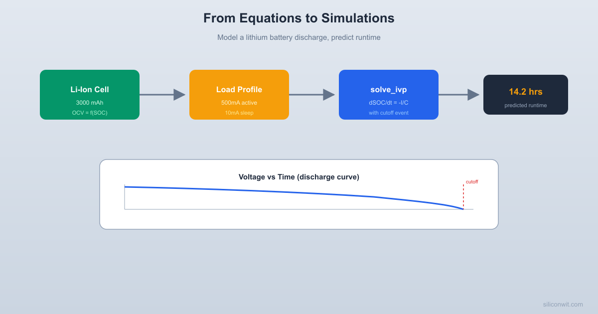
Battery Discharge Simulator
Models a lithium-ion cell under a variable load profile.
Predicts voltage, SOC, and runtime.
from scipy.integrate import solve_ivp
import matplotlib.pyplot as plt
# -------------------------------------------------------
# -------------------------------------------------------
CAPACITY_AH = 3.0 # Cell capacity in Ah
R_INTERNAL = 0.05 # Internal resistance in ohms
V_CUTOFF = 3.0 # Cutoff voltage in V
# OCV polynomial coefficients (fit to a typical 18650 curve)
# V_ocv(SOC) = a0 + a1*SOC + a2*SOC^2 + a3*SOC^3
OCV_COEFFS = [3.0, 0.55, 0.95, -0.30]
"""Open-circuit voltage as a function of state of charge."""
soc_clipped = np.clip(soc, 0.0, 1.0)
return a[0] + a[1]*soc_clipped + a[2]*soc_clipped**2 + a[3]*soc_clipped**3
def terminal_voltage(soc, current_a):
"""Terminal voltage under load (OCV minus resistive drop)."""
return ocv_from_soc(soc) - current_a * R_INTERNAL
# -------------------------------------------------------
# -------------------------------------------------------
SLEEP_CURRENT_A = 0.010 # 10 mA during sleep
ACTIVE_CURRENT_A = 0.500 # 500 mA during active burst
ACTIVE_DURATION_S = 2.0 # Active burst lasts 2 seconds
CYCLE_PERIOD_S = 10.0 # One full sleep+active cycle
Returns the load current in amperes at time t (seconds).
Repeating pattern: active burst for ACTIVE_DURATION_S,
then sleep for the remainder of the cycle.
phase = t % CYCLE_PERIOD_S
if phase < ACTIVE_DURATION_S:
# -------------------------------------------------------
# ODE: dSOC/dt = -I(t) / (Q * 3600)
# Note: Q is in Ah, t is in seconds, so we divide by 3600
# -------------------------------------------------------
"""State equation for battery discharge."""
current = load_current(t)
dsoc_dt = -current / (CAPACITY_AH * 3600.0)
# -------------------------------------------------------
# Event: stop when terminal voltage hits cutoff
# -------------------------------------------------------
def voltage_cutoff_event(t, y):
"""Returns zero when terminal voltage reaches V_CUTOFF."""
current = load_current(t)
v_term = terminal_voltage(soc, current)
voltage_cutoff_event.terminal = True
voltage_cutoff_event.direction = -1
# -------------------------------------------------------
# -------------------------------------------------------
"""Simulate battery discharge and plot results."""
soc_initial = 1.0 # Start fully charged
t_max = 200000.0 # Maximum simulation time (seconds)
print(" BATTERY DISCHARGE SIMULATOR")
print(f" Cell capacity: {CAPACITY_AH:.1f} Ah ({CAPACITY_AH*1000:.0f} mAh)")
print(f" Internal resistance: {R_INTERNAL*1000:.0f} mohm")
print(f" Cutoff voltage: {V_CUTOFF:.1f} V")
print(f" Sleep current: {SLEEP_CURRENT_A*1000:.0f} mA")
print(f" Active current: {ACTIVE_CURRENT_A*1000:.0f} mA")
print(f" Duty cycle: {ACTIVE_DURATION_S/CYCLE_PERIOD_S*100:.0f}%")
avg_current = (ACTIVE_CURRENT_A * ACTIVE_DURATION_S +
SLEEP_CURRENT_A * (CYCLE_PERIOD_S - ACTIVE_DURATION_S)) / CYCLE_PERIOD_S
print(f" Average current: {avg_current*1000:.0f} mA")
events=voltage_cutoff_event,
max_step=1.0, # Sample at least every 1 second
# Generate smooth time vector for plotting
t_plot = np.linspace(0, t_end, 2000)
soc_plot = sol.sol(t_plot)[0]
# Compute voltage at each time point
v_plot = np.array([terminal_voltage(s, load_current(t))
for s, t in zip(soc_plot, t_plot)])
# Compute current at each time point (for reference)
i_plot = np.array([load_current(t) for t in t_plot])
# Convert time to hours for plotting
t_hours = t_plot / 3600.0
runtime_hours = t_end / 3600.0
print(f" Predicted runtime: {runtime_hours:.1f} hours")
print(f" Final SOC: {final_soc*100:.1f}%")
print(f" Final voltage: {v_plot[-1]:.2f} V")
# Simple estimate for comparison
simple_hours = CAPACITY_AH / avg_current
print(f" Simple estimate: {simple_hours:.1f} hours (capacity / avg current)")
print(f" Difference: {abs(runtime_hours - simple_hours):.1f} hours")
# -------------------------------------------------------
# -------------------------------------------------------
fig, axes = plt.subplots(3, 1, figsize=(10, 8), sharex=True)
fig.suptitle("Battery Discharge Simulation", fontsize=14, fontweight="bold")
# Plot 1: Terminal voltage
axes[0].plot(t_hours, v_plot, color="tab:blue", linewidth=1.5)
axes[0].axhline(y=V_CUTOFF, color="red", linestyle="--", alpha=0.7,
label=f"Cutoff ({V_CUTOFF} V)")
axes[0].set_ylabel("Terminal Voltage (V)")
axes[0].set_ylim([2.8, 4.4])
axes[0].legend(loc="upper right")
axes[0].grid(True, alpha=0.3)
# Plot 2: State of charge
axes[1].plot(t_hours, soc_plot * 100, color="tab:green", linewidth=1.5)
axes[1].set_ylabel("State of Charge (%)")
axes[1].set_ylim([-5, 105])
axes[1].grid(True, alpha=0.3)
# Downsample for current plot (it's a square wave)
t_current = np.linspace(0, min(t_end, 60), 1000) # Show first 60 seconds
i_current = np.array([load_current(t) * 1000 for t in t_current])
axes[2].plot(t_current, i_current, color="tab:orange", linewidth=1.0)
axes[2].set_ylabel("Load Current (mA)")
axes[2].set_xlabel("Time (seconds, first 60 s shown)")
axes[2].set_ylim([-50, 600])
axes[2].grid(True, alpha=0.3)
plt.savefig("battery_discharge.png", dpi=150, bbox_inches="tight")
print("\nPlot saved as battery_discharge.png")
if __name__ == "__main__":
Comments