Real-Time Dashboards and Data Visualization

Modified: Mar. 14, 2026

Published: Mar. 10, 2026

Become Contributor Expert Support

Your MQTT broker is routing sensor data, and your MCU clients are publishing JSON payloads on a schedule. But data flowing through a broker is invisible unless you store it and visualize it. In this lesson you will build a complete MQTT-to-dashboard pipeline using Telegraf, InfluxDB, and Grafana (the TIG stack), then compare it with the managed dashboards on SiliconWit.io, and finally build a lightweight Chart.js alternative for resource-constrained gateways. #Dashboard #Grafana #DataViz

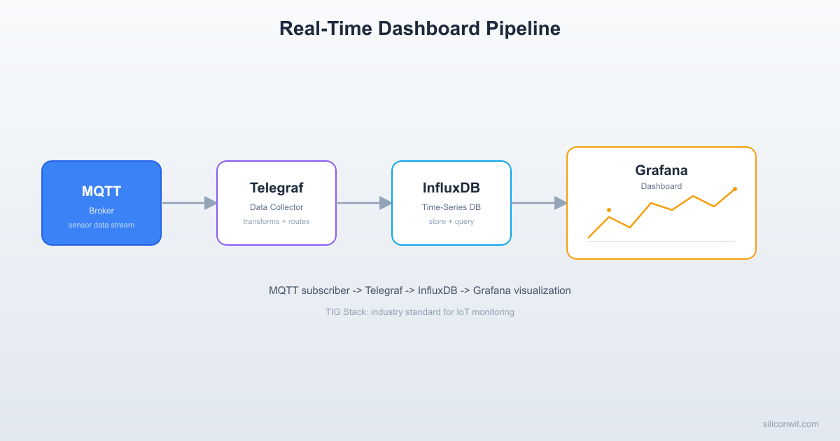
The MQTT-to-Dashboard Pipeline

The pipeline has four stages, each handled by a dedicated tool:

  TIG Stack Data Flow
  ──────────────────────────────────────────
  Sensor ──► Mosquitto ──► Telegraf ──► InfluxDB
  (MQTT       (broker)    (MQTT sub     (time-
   publish)               + parser)     series DB)
                                           │
                                           │ Flux
                                           │ query
                                           ▼
                                        Grafana
                                        (panels:
                                         line chart,
                                         gauge,
                                         table,
                                         alerts)

  Each component is independent. If Grafana
  goes down, data keeps flowing into InfluxDB.

Data flows in one direction: sensor publishes to Mosquitto, Telegraf consumes the message, writes it to InfluxDB, and Grafana queries InfluxDB on a refresh interval (typically every 5 seconds). Each component is independent. If Grafana goes down, data keeps flowing into InfluxDB. If Telegraf restarts, it reconnects to the broker and resumes ingestion.

Installing the TIG Stack

You can install all four components (Mosquitto + Telegraf + InfluxDB + Grafana) either through system packages or through Docker Compose. Docker is the recommended approach because it isolates each service, makes upgrades trivial, and produces the same environment on any Linux distribution.

  Grafana Dashboard Panel Layout
  ──────────────────────────────────────────
  ┌──────────────────────────────────────┐
  │ Temperature (Line Chart)             │
  │  30C ─────────╱╲──────────           │
  │  25C ────────╱──╲─────────           │
  │  20C ───────╱────╲────────           │
  │       0h    6h   12h   18h   24h     │
  ├──────────────┬───────────────────────┤
  │  Humidity    │  Pressure  │ Status   │
  │  ┌─────┐    │  1013 hPa  │ Node 1 ✓│
  │  │ 65% │    │  ┌──────┐  │ Node 2 ✓│
  │  │gauge│    │  │ stat  │  │ Node 3 ✗│
  │  └─────┘    │  └──────┘  │          │
  └──────────────┴───────────┴──────────┘

sudo apt update
sudo apt install -y docker.io docker-compose-v2
sudo usermod -aG docker $USER
# Log out and back in for the group change to take effect

version: "3.8"

services:
  mosquitto:
    image: eclipse-mosquitto:2
    container_name: mosquitto
    ports:
      - "1883:1883"
      - "9001:9001"
    volumes:
      - ./mosquitto/config:/mosquitto/config
      - ./mosquitto/data:/mosquitto/data
      - ./mosquitto/log:/mosquitto/log
    restart: unless-stopped

  telegraf:
    image: telegraf:1.32
    container_name: telegraf
    depends_on:
      - mosquitto
      - influxdb
    volumes:
      - ./telegraf/telegraf.conf:/etc/telegraf/telegraf.conf:ro
    restart: unless-stopped

  influxdb:
    image: influxdb:2.7
    container_name: influxdb
    ports:
      - "8086:8086"
    volumes:
      - influxdb-data:/var/lib/influxdb2
      - influxdb-config:/etc/influxdb2
    environment:
      - DOCKER_INFLUXDB_INIT_MODE=setup
      - DOCKER_INFLUXDB_INIT_USERNAME=admin
      - DOCKER_INFLUXDB_INIT_PASSWORD=changeme1234
      - DOCKER_INFLUXDB_INIT_ORG=siliconwit
      - DOCKER_INFLUXDB_INIT_BUCKET=iot_sensors
      - DOCKER_INFLUXDB_INIT_RETENTION=30d
      - DOCKER_INFLUXDB_INIT_ADMIN_TOKEN=my-super-secret-token
    restart: unless-stopped

  grafana:
    image: grafana/grafana:11.2.0
    container_name: grafana
    ports:
      - "3000:3000"
    volumes:
      - grafana-data:/var/lib/grafana
    environment:
      - GF_SECURITY_ADMIN_USER=admin
      - GF_SECURITY_ADMIN_PASSWORD=admin
    depends_on:
      - influxdb
    restart: unless-stopped

volumes:
  influxdb-data:
  influxdb-config:
  grafana-data:

mkdir -p mosquitto/config mosquitto/data mosquitto/log

listener 1883
allow_anonymous true
persistence true
persistence_location /mosquitto/data/
log_dest file /mosquitto/log/mosquitto.log

docker compose up -d

docker compose ps

sudo apt update
sudo apt install -y mosquitto mosquitto-clients
sudo systemctl enable mosquitto
sudo systemctl start mosquitto

# Add the InfluxData GPG key and repository
curl -sL https://repos.influxdata.com/influxdata-archive.key | sudo gpg --dearmor -o /etc/apt/trusted.gpg.d/influxdata.gpg
echo "deb https://repos.influxdata.com/debian stable main" | sudo tee /etc/apt/sources.list.d/influxdata.list

sudo apt update
sudo apt install -y influxdb2
sudo systemctl enable influxdb
sudo systemctl start influxdb

influx setup \
  --username admin \
  --password changeme1234 \
  --org siliconwit \
  --bucket iot_sensors \
  --retention 30d \
  --token my-super-secret-token \
  --force

sudo apt install -y telegraf
sudo systemctl enable telegraf

sudo apt install -y apt-transport-https software-properties-common
curl -sL https://apt.grafana.com/gpg.key | sudo gpg --dearmor -o /etc/apt/trusted.gpg.d/grafana.gpg
echo "deb https://apt.grafana.com stable main" | sudo tee /etc/apt/sources.list.d/grafana.list

sudo apt update
sudo apt install -y grafana
sudo systemctl enable grafana-server
sudo systemctl start grafana-server

sudo systemctl status mosquitto influxdb telegraf grafana-server

Configuring Telegraf as the MQTT Consumer

Telegraf is the glue between your MQTT broker and InfluxDB. It subscribes to MQTT topics, parses the incoming JSON payloads, and writes structured measurements to InfluxDB. The entire behavior is controlled by a single configuration file.

Telegraf Configuration File

mkdir -p telegraf

# Global agent configuration
[agent]
  interval = "10s"
  round_interval = true
  metric_batch_size = 1000
  metric_buffer_limit = 10000
  flush_interval = "10s"
  flush_jitter = "0s"

# InfluxDB v2 output plugin
[[outputs.influxdb_v2]]
  urls = ["http://influxdb:8086"]
  token = "my-super-secret-token"
  organization = "siliconwit"
  bucket = "iot_sensors"

# MQTT consumer input plugin
[[inputs.mqtt_consumer]]
  servers = ["tcp://mosquitto:1883"]
  topics = [
    "sensors/#",
    "home/#",
    "factory/#"
  ]
  qos = 1
  connection_timeout = "30s"
  persistent_session = false
  client_id = "telegraf-subscriber"

  # Parse JSON payloads
  data_format = "json"

  # Use the MQTT topic as the measurement name
  # For topic "sensors/esp32-01/bme280", the measurement becomes "mqtt_consumer"
  # and we extract tags from the topic path
  [[inputs.mqtt_consumer.topic_parsing]]
    topic = "sensors/+/+"
    measurement = "measurement/_/_"
    tags = "_/device/sensor_type"

  [[inputs.mqtt_consumer.topic_parsing]]
    topic = "home/+/+"
    measurement = "measurement/_/_"
    tags = "_/location/reading_type"

  [[inputs.mqtt_consumer.topic_parsing]]
    topic = "factory/+/+"
    measurement = "measurement/_/_"
    tags = "_/zone/metric"

docker compose restart telegraf

# Global agent configuration
[agent]
  interval = "10s"
  round_interval = true
  metric_batch_size = 1000
  metric_buffer_limit = 10000
  flush_interval = "10s"
  flush_jitter = "0s"

# InfluxDB v2 output plugin
[[outputs.influxdb_v2]]
  urls = ["http://localhost:8086"]
  token = "my-super-secret-token"
  organization = "siliconwit"
  bucket = "iot_sensors"

# MQTT consumer input plugin
[[inputs.mqtt_consumer]]
  servers = ["tcp://localhost:1883"]
  topics = [
    "sensors/#",
    "home/#",
    "factory/#"
  ]
  qos = 1
  connection_timeout = "30s"
  persistent_session = false
  client_id = "telegraf-subscriber"

  # Parse JSON payloads
  data_format = "json"

  # Extract tags from MQTT topic hierarchy
  [[inputs.mqtt_consumer.topic_parsing]]
    topic = "sensors/+/+"
    measurement = "measurement/_/_"
    tags = "_/device/sensor_type"

  [[inputs.mqtt_consumer.topic_parsing]]
    topic = "home/+/+"
    measurement = "measurement/_/_"
    tags = "_/location/reading_type"

  [[inputs.mqtt_consumer.topic_parsing]]
    topic = "factory/+/+"
    measurement = "measurement/_/_"
    tags = "_/zone/metric"

sudo systemctl restart telegraf

Understanding the Configuration

The configuration has three main sections:

Agent settings. The interval controls how often Telegraf collects data from its inputs. For MQTT this is less relevant because messages arrive asynchronously, but it affects other input plugins. The flush_interval controls how often Telegraf writes batched metrics to the output (InfluxDB).

Output plugin. The influxdb_v2 output sends data to InfluxDB 2.x. The token authenticates the connection. The organization and bucket specify where data lands. In Docker, the URL uses the container name (influxdb) instead of localhost because Docker Compose creates an internal network.

Input plugin. The mqtt_consumer subscribes to the specified topics with QoS 1. The data_format = "json" tells Telegraf to parse each MQTT payload as JSON. Every key in the JSON object becomes a field in InfluxDB.

Topic parsing. This is the most powerful part. Without topic parsing, every MQTT message lands in a single measurement called mqtt_consumer with no device or location tags. The topic_parsing blocks extract structured tags from the topic hierarchy. For example, a message on sensors/esp32-01/bme280 creates a measurement named sensors with tags device=esp32-01 and sensor_type=bme280. This makes it possible to filter and group data by device or sensor type in Grafana.

Verify Data Ingestion

Publish a test message from the command line and check that it arrives in InfluxDB:

mosquitto_pub -h localhost -t "sensors/esp32-test/bme280" \
  -m '{"temperature": 24.5, "humidity": 62.3, "pressure": 1013.2}'

Wait 10 seconds (one flush interval), then query InfluxDB:

influx query '
  from(bucket: "iot_sensors")
  |> range(start: -5m)
  |> filter(fn: (r) => r["device"] == "esp32-test")
' --org siliconwit --token my-super-secret-token

You should see one row with temperature, humidity, and pressure fields, tagged with device=esp32-test and sensor_type=bme280.

InfluxDB Fundamentals

Before building dashboards, you need to understand how InfluxDB organizes data. InfluxDB 2.x uses a different data model than traditional relational databases.

Core Concepts

Bucket. A bucket is where time-series data is stored. It is similar to a database in SQL terms. Each bucket has a retention policy that automatically deletes data older than a specified duration. Our iot_sensors bucket retains data for 30 days.

Measurement. A measurement is analogous to a table. Each measurement holds data points that share the same name. With our Telegraf topic parsing, the measurement name comes from the first segment of the MQTT topic (e.g., sensors, home, factory).

Tags. Tags are indexed key-value pairs used for filtering and grouping. They describe metadata about the data point: which device sent it, which location it came from, what type of sensor produced it. Tags are strings and are always indexed, making tag-based queries fast.

Fields. Fields hold the actual measured values: temperature, humidity, pressure, voltage. Fields are not indexed, which means filtering by field value requires scanning all matching data points. Fields can be floats, integers, strings, or booleans.

Timestamp. Every data point has a nanosecond-precision timestamp. If the MQTT payload does not include a timestamp, Telegraf stamps it with the current time when the message arrives.

Tags vs Fields: When to Use Each

The rule of thumb: if you will filter or group by it, make it a tag. If you will plot or aggregate it, make it a field.

Retention Policies

Retention policies control how long data is kept. For IoT, a common pattern is to keep raw data for a short period and downsampled data for longer:

You can create additional buckets and use InfluxDB tasks (scheduled Flux scripts) to downsample data automatically. We will set up a downsampling task later in this lesson.

Flux Query Language

InfluxDB 2.x uses Flux as its query language. Flux is a functional, pipe-based language where each step transforms the data and passes it to the next step.

Here is a basic query that retrieves the last hour of temperature data from a specific device:

from(bucket: "iot_sensors")
  |> range(start: -1h)
  |> filter(fn: (r) => r["_measurement"] == "sensors")
  |> filter(fn: (r) => r["device"] == "esp32-01")
  |> filter(fn: (r) => r["_field"] == "temperature")

Each line does one thing:

1. from(bucket:) selects the data source.
2. range(start:) limits the time window. Every Flux query requires a range.
3. filter(fn:) narrows the results by measurement, tags, or fields.

The |> operator pipes the output of one function into the input of the next, similar to Unix pipes.

Aggregating by Time Window

To calculate the average temperature in 5-minute windows:

from(bucket: "iot_sensors")
  |> range(start: -6h)
  |> filter(fn: (r) => r["_measurement"] == "sensors")
  |> filter(fn: (r) => r["device"] == "esp32-01")
  |> filter(fn: (r) => r["_field"] == "temperature")
  |> aggregateWindow(every: 5m, fn: mean, createEmpty: false)

The aggregateWindow function groups data points into 5-minute buckets and applies the mean function to each bucket. Setting createEmpty: false prevents empty windows from appearing in the output when no data was received during that interval.

Comparing Multiple Devices

To plot data from multiple devices on the same chart:

from(bucket: "iot_sensors")
  |> range(start: -1h)
  |> filter(fn: (r) => r["_measurement"] == "sensors")
  |> filter(fn: (r) => r["_field"] == "temperature")
  |> aggregateWindow(every: 1m, fn: mean, createEmpty: false)

By removing the device filter, this query returns temperature data from all devices. Grafana automatically groups the results by the device tag and plots each device as a separate line on the chart.

Detecting Anomalies

A simple anomaly detection query that flags readings outside a normal range:

from(bucket: "iot_sensors")
  |> range(start: -1h)
  |> filter(fn: (r) => r["_measurement"] == "sensors")
  |> filter(fn: (r) => r["_field"] == "temperature")
  |> filter(fn: (r) => r["_value"] > 40.0 or r["_value"] < 0.0)

This returns only data points where the temperature is above 40 degrees or below 0 degrees. You can use this kind of query in Grafana alerts to trigger notifications when sensor readings leave the expected range.

Downsampling Task

Create a scheduled task that downsamples raw data into 5-minute averages:

option task = {name: "downsample_5m", every: 10m}

from(bucket: "iot_sensors")
  |> range(start: -10m)
  |> filter(fn: (r) => r["_measurement"] == "sensors")
  |> aggregateWindow(every: 5m, fn: mean, createEmpty: false)
  |> to(bucket: "iot_sensors_weekly", org: "siliconwit")

This task runs every 10 minutes, reads the last 10 minutes of raw data, computes 5-minute averages, and writes the results to the iot_sensors_weekly bucket (which you would create with a 365-day retention policy).

Setting Up Grafana

Grafana is the visualization layer. It connects to InfluxDB, runs Flux queries, and renders the results as interactive panels on a dashboard.

Add InfluxDB as a Data Source

1. Open Grafana at http://localhost:3000 and log in (default: admin / admin). Grafana will prompt you to change the password on first login.

2. Navigate to Connections in the left sidebar, then click Data sources.

3. Click Add data source and select InfluxDB.

4. Configure the data source with these settings:

   Setting	Value
   Query Language	Flux
   URL	http://influxdb:8086 (Docker) or http://localhost:8086 (apt)
   Organization	siliconwit
   Token	my-super-secret-token
   Default Bucket	iot_sensors

5. Click Save & Test. You should see a green “Data source is working” confirmation.

Create a Dashboard

1. Click the + icon in the left sidebar and select New dashboard.

2. Click Add visualization to create your first panel.

3. In the query editor at the bottom, select the InfluxDB data source you just configured.

4. Switch to the Script Editor (click the pencil icon) and paste a Flux query.

5. Click Run query to preview the data, then adjust the panel settings in the right sidebar.

6. Click Apply to add the panel to the dashboard.

7. Repeat for each additional panel. Arrange panels by dragging and resizing.

8. Click the Save icon (disk icon) in the top toolbar and name your dashboard “IoT Sensor Dashboard”.

Auto-Refresh

Click the refresh interval dropdown in the top-right corner of the dashboard and select 5s for a near-real-time experience. Grafana will re-run all panel queries every 5 seconds.

Building Dashboard Panels

A well-designed IoT dashboard uses different panel types for different purposes. Here are the five most useful panel types for sensor data.

1. Time Series (Line Chart)

The most common panel type for IoT. It plots values over time, with one line per device or sensor.

Use case: Temperature, humidity, and pressure over the last 6 hours.

from(bucket: "iot_sensors")
  |> range(start: v.timeRangeStart, stop: v.timeRangeStop)
  |> filter(fn: (r) => r["_measurement"] == "sensors")
  |> filter(fn: (r) => r["_field"] == "temperature")
  |> aggregateWindow(every: v.windowPeriod, fn: mean, createEmpty: false)

The variables v.timeRangeStart, v.timeRangeStop, and v.windowPeriod are provided by Grafana and automatically adjust when you change the dashboard time range or zoom into a section of the chart.

Panel settings:

• Title: “Temperature Over Time”
• Unit: Celsius (under Standard options, set Unit to “Temperature / Celsius”)
• Thresholds: Add a red threshold at 40 to highlight overheating
• Legend: Show as table, display Min, Max, and Last values

2. Gauge Panel

A gauge shows a single current value against a defined range. Good for readings that have well-known limits.

Use case: Current humidity level from one sensor.

from(bucket: "iot_sensors")
  |> range(start: -5m)
  |> filter(fn: (r) => r["_measurement"] == "sensors")
  |> filter(fn: (r) => r["device"] == "esp32-01")
  |> filter(fn: (r) => r["_field"] == "humidity")
  |> last()

The last() function returns only the most recent data point.

Panel settings:

• Title: “Humidity”
• Min: 0, Max: 100
• Thresholds: Green (0-30), Yellow (30-70), Red (70-100)
• Unit: Humidity / %H

3. Stat Panel

A stat panel displays a single large number with optional sparkline. It is useful for at-a-glance readings.

Use case: Latest temperature reading from a device.

from(bucket: "iot_sensors")
  |> range(start: -5m)
  |> filter(fn: (r) => r["_measurement"] == "sensors")
  |> filter(fn: (r) => r["device"] == "esp32-01")
  |> filter(fn: (r) => r["_field"] == "temperature")
  |> last()

Panel settings:

• Title: “Temperature Now”
• Graph mode: Area (shows a small sparkline behind the number)
• Color mode: From thresholds
• Thresholds: Green (base), Orange (35), Red (40)

4. Table Panel

A table shows structured data in rows and columns. Good for showing recent events or a summary of all devices.

Use case: Last 20 sensor readings with device, timestamp, and all fields.

from(bucket: "iot_sensors")
  |> range(start: -30m)
  |> filter(fn: (r) => r["_measurement"] == "sensors")
  |> pivot(rowKey: ["_time"], columnKey: ["_field"], valueColumn: "_value")
  |> sort(columns: ["_time"], desc: true)
  |> limit(n: 20)

The pivot function transforms the data so that each field (temperature, humidity, pressure) becomes its own column instead of separate rows. This produces a clean table with one row per timestamp.

Panel settings:

• Title: “Recent Readings”
• Column widths: Auto
• Cell display: Color text for temperature column (with thresholds)

5. Alert List Panel

An alert list panel shows the current state of all configured alerts. It provides a summary view of which alerts are firing, pending, or normal.

Panel settings:

• Title: “Active Alerts”
• Show: Current alerts
• State filter: Alerting, Pending
• Sort by: Time (newest first)

We will configure the actual alert rules in Lesson 6. For now, you can add this panel as a placeholder so the dashboard layout is ready.

Example Dashboard Layout

Here is a recommended layout for an IoT sensor dashboard. Arrange the panels in a grid:

To make a panel span the full width, drag its right edge to the edge of the dashboard. Grafana uses a 24-column grid, so a full-width panel is 24 units wide.

Adding Threshold Lines to Time Series

Threshold lines on a time series chart make it immediately obvious when values enter a danger zone:

1. Edit the Temperature time series panel.
2. In the right sidebar, scroll down to Thresholds.
3. Add a threshold at 40 with color Red and label “Max Safe”.
4. Add a threshold at 5 with color Blue and label “Min Safe”.
5. Under Threshold display, select As lines (instead of the default “As filled regions”).
6. Click Apply.

The chart now shows horizontal lines at 40 and 5 degrees. Any data points above or below these lines stand out visually.

Device Grouping with Template Variables

When you have multiple devices, you do not want separate dashboards for each one. Instead, use a Grafana template variable to create a device selector dropdown:

1. Open the dashboard settings (gear icon in the top toolbar).

2. Click Variables in the left menu.

3. Click Add variable and configure it:

   Setting	Value
   Name	device
   Type	Query
   Data source	InfluxDB
   Query	import "influxdata/influxdb/schema" then schema.tagValues(bucket: "iot_sensors", tag: "device")
   Multi-value	Enabled
   Include All option	Enabled

4. Click Apply.

Now update your panel queries to use the variable:

from(bucket: "iot_sensors")
  |> range(start: v.timeRangeStart, stop: v.timeRangeStop)
  |> filter(fn: (r) => r["_measurement"] == "sensors")
  |> filter(fn: (r) => r["device"] == "${device}")
  |> filter(fn: (r) => r["_field"] == "temperature")
  |> aggregateWindow(every: v.windowPeriod, fn: mean, createEmpty: false)

A dropdown appears at the top of the dashboard. Selecting a device filters all panels instantly.

SiliconWit.io Dashboard Comparison

The TIG stack gives you full control, but it requires a Linux server, Docker, and ongoing maintenance. For projects where you want dashboards without managing infrastructure, SiliconWit.io provides a managed alternative.

How SiliconWit.io Works

Your MQTT clients connect to SiliconWit.io’s MQTT endpoint (or your own broker with cloud forwarding configured), and the platform handles storage, visualization, and alerting automatically. There is no Telegraf or InfluxDB to install.

Viewing Data on SiliconWit.io

If you already created a SiliconWit.io account (from the Getting Started section of the course index), your sensor data is already flowing to the platform if your MCU clients are configured to publish to SiliconWit.io’s MQTT endpoint.

The SiliconWit.io dashboard provides:

• Live charts that update in real time as new sensor data arrives
• Data tables showing individual readings with timestamps and device metadata
• Exportable reports in CSV format for analysis in spreadsheets or Python
• Device overview showing online/offline status for all connected devices
• Historical data browsing with adjustable time ranges

When to Use Each Approach

Use SiliconWit.io when:

• You want dashboards running in under 5 minutes
• You do not have a dedicated Linux server
• You are prototyping or building a small deployment (under 10 devices)
• You want built-in alerting without configuring Grafana alert rules

Use the self-hosted TIG stack when:

• You need full control over data storage and retention
• You have specific compliance or data sovereignty requirements
• You want custom Grafana plugins or advanced visualization
• You are building a large-scale deployment with dozens of devices
• You need to integrate with internal systems that cannot reach the public internet

You can also use both: self-hosted Grafana for detailed engineering analysis and SiliconWit.io for stakeholder-facing dashboards that require no maintenance.

Lightweight Dashboard with Chart.js

Not every IoT gateway has the resources to run Grafana. A Raspberry Pi Zero or an OpenWrt router can serve a simple web dashboard using Chart.js, a lightweight JavaScript charting library that runs entirely in the browser. This is useful for local monitoring when you need a quick visual without cloud connectivity.

Project Structure

iot-dashboard/
  index.html
  style.css
  app.js

HTML Page

<!DOCTYPE html>
<html lang="en">
<head>
  <meta charset="UTF-8">
  <meta name="viewport" content="width=device-width, initial-scale=1.0">
  <title>IoT Sensor Dashboard</title>
  <link rel="stylesheet" href="style.css">
  <script src="https://cdn.jsdelivr.net/npm/[email protected]"></script>
  <script src="https://cdn.jsdelivr.net/npm/[email protected]/dist/mqtt.min.js"></script>
</head>
<body>
  <h1>IoT Sensor Dashboard</h1>
  <div class="stats">
    <div class="stat-card">
      <span class="stat-label">Temperature</span>
      <span class="stat-value" id="temp-value">--</span>
      <span class="stat-unit">&deg;C</span>
    </div>
    <div class="stat-card">
      <span class="stat-label">Humidity</span>
      <span class="stat-value" id="hum-value">--</span>
      <span class="stat-unit">%</span>
    </div>
    <div class="stat-card">
      <span class="stat-label">Pressure</span>
      <span class="stat-value" id="pres-value">--</span>
      <span class="stat-unit">hPa</span>
    </div>
  </div>
  <div class="chart-container">
    <canvas id="tempChart"></canvas>
  </div>
  <div class="chart-container">
    <canvas id="humChart"></canvas>
  </div>
  <script src="app.js"></script>
</body>
</html>

CSS Styling

* { margin: 0; padding: 0; box-sizing: border-box; }
body {
  font-family: system-ui, sans-serif;
  background: #1a1a2e;
  color: #eee;
  padding: 20px;
}
h1 {
  text-align: center;
  margin-bottom: 20px;
  font-size: 1.5rem;
}
.stats {
  display: flex;
  gap: 16px;
  justify-content: center;
  margin-bottom: 24px;
  flex-wrap: wrap;
}
.stat-card {
  background: #16213e;
  border-radius: 8px;
  padding: 16px 24px;
  text-align: center;
  min-width: 140px;
}
.stat-label {
  display: block;
  font-size: 0.85rem;
  color: #aaa;
  margin-bottom: 4px;
}
.stat-value {
  display: block;
  font-size: 2rem;
  font-weight: bold;
  color: #0f3460;
}
.stat-unit {
  font-size: 0.9rem;
  color: #888;
}
.chart-container {
  background: #16213e;
  border-radius: 8px;
  padding: 16px;
  margin-bottom: 16px;
  max-width: 800px;
  margin-left: auto;
  margin-right: auto;
}

JavaScript Application

// Configuration
const BROKER_URL = "ws://localhost:9001";  // Mosquitto WebSocket port
const TOPIC = "sensors/#";
const MAX_POINTS = 60;  // Keep last 60 data points on chart

// Chart.js setup for temperature
const tempCtx = document.getElementById("tempChart").getContext("2d");
const tempChart = new Chart(tempCtx, {
  type: "line",
  data: {
    labels: [],
    datasets: [{
      label: "Temperature (C)",
      data: [],
      borderColor: "#e94560",
      backgroundColor: "rgba(233, 69, 96, 0.1)",
      fill: true,
      tension: 0.3,
      pointRadius: 2,
    }],
  },
  options: {
    responsive: true,
    animation: { duration: 300 },
    scales: {
      x: {
        ticks: { color: "#888", maxTicksLimit: 10 },
        grid: { color: "#333" },
      },
      y: {
        ticks: { color: "#888" },
        grid: { color: "#333" },
        suggestedMin: 15,
        suggestedMax: 45,
      },
    },
    plugins: {
      legend: { labels: { color: "#ccc" } },
      annotation: {
        annotations: {
          threshold: {
            type: "line",
            yMin: 40,
            yMax: 40,
            borderColor: "red",
            borderWidth: 1,
            borderDash: [6, 4],
            label: {
              content: "Max Safe",
              enabled: true,
              position: "start",
            },
          },
        },
      },
    },
  },
});

// Chart.js setup for humidity
const humCtx = document.getElementById("humChart").getContext("2d");
const humChart = new Chart(humCtx, {
  type: "line",
  data: {
    labels: [],
    datasets: [{
      label: "Humidity (%)",
      data: [],
      borderColor: "#0f3460",
      backgroundColor: "rgba(15, 52, 96, 0.1)",
      fill: true,
      tension: 0.3,
      pointRadius: 2,
    }],
  },
  options: {
    responsive: true,
    animation: { duration: 300 },
    scales: {
      x: {
        ticks: { color: "#888", maxTicksLimit: 10 },
        grid: { color: "#333" },
      },
      y: {
        ticks: { color: "#888" },
        grid: { color: "#333" },
        suggestedMin: 0,
        suggestedMax: 100,
      },
    },
    plugins: {
      legend: { labels: { color: "#ccc" } },
    },
  },
});

// Helper: add a data point to a chart, removing old points if needed
function addDataPoint(chart, label, value) {
  chart.data.labels.push(label);
  chart.data.datasets[0].data.push(value);
  if (chart.data.labels.length > MAX_POINTS) {
    chart.data.labels.shift();
    chart.data.datasets[0].data.shift();
  }
  chart.update();
}

// Format timestamp for chart labels
function timeLabel() {
  const now = new Date();
  return now.toLocaleTimeString("en-GB", {
    hour: "2-digit",
    minute: "2-digit",
    second: "2-digit",
  });
}

// Connect to MQTT over WebSocket
const client = mqtt.connect(BROKER_URL);

client.on("connect", () => {
  console.log("Connected to MQTT broker");
  client.subscribe(TOPIC, { qos: 1 });
});

client.on("message", (topic, message) => {
  try {
    const data = JSON.parse(message.toString());
    const label = timeLabel();

    if (data.temperature !== undefined) {
      document.getElementById("temp-value").textContent =
        data.temperature.toFixed(1);
      addDataPoint(tempChart, label, data.temperature);
    }
    if (data.humidity !== undefined) {
      document.getElementById("hum-value").textContent =
        data.humidity.toFixed(1);
      addDataPoint(humChart, label, data.humidity);
    }
    if (data.pressure !== undefined) {
      document.getElementById("pres-value").textContent =
        data.pressure.toFixed(0);
    }
  } catch (err) {
    console.error("Failed to parse MQTT message:", err);
  }
});

client.on("error", (err) => {
  console.error("MQTT connection error:", err);
});

Enabling WebSocket on Mosquitto

The browser MQTT client connects over WebSocket, so Mosquitto needs a WebSocket listener. Add this to your Mosquitto configuration:

listener 9001
protocol websockets

If you are using the Docker Compose setup from earlier, the port mapping 9001:9001 is already included. Just add the WebSocket listener to the config file and restart Mosquitto:

docker compose restart mosquitto

Serve the Dashboard

You can serve the static files with any HTTP server. Python’s built-in server works for development:

cd iot-dashboard
python3 -m http.server 8080

Open http://localhost:8080 in a browser. As MQTT messages arrive, the stat cards update and the charts scroll with live data. This entire dashboard is three files totaling under 5 KB (excluding the CDN-loaded libraries).

Data Export

Dashboards are great for real-time monitoring, but you often need to extract data for analysis, reporting, or archival purposes.

CSV Export from Grafana

Grafana can export any panel’s data as CSV:

1. Hover over a panel and click the three-dot menu icon.
2. Select Inspect then Data.
3. Click Download CSV.

The exported CSV includes timestamps, tags, and field values for the queried time range.

CSV Export via InfluxDB CLI

For automated or scripted exports, use the InfluxDB CLI with the --raw flag to get CSV output:

influx query '
  from(bucket: "iot_sensors")
  |> range(start: -24h)
  |> filter(fn: (r) => r["_measurement"] == "sensors")
  |> filter(fn: (r) => r["_field"] == "temperature")
  |> pivot(rowKey: ["_time"], columnKey: ["_field"], valueColumn: "_value")
' --org siliconwit --token my-super-secret-token --raw > temperature_export.csv

API Queries

InfluxDB exposes a REST API for programmatic access. You can query data from any language that can make HTTP requests:

curl -s -XPOST "http://localhost:8086/api/v2/query?org=siliconwit" \
  -H "Authorization: Token my-super-secret-token" \
  -H "Content-Type: application/vnd.flux" \
  -d 'from(bucket: "iot_sensors")
       |> range(start: -1h)
       |> filter(fn: (r) => r["_field"] == "temperature")
       |> last()'

A Python example using the official InfluxDB client:

from influxdb_client import InfluxDBClient

client = InfluxDBClient(
    url="http://localhost:8086",
    token="my-super-secret-token",
    org="siliconwit",
)

query_api = client.query_api()

query = '''
from(bucket: "iot_sensors")
  |> range(start: -1h)
  |> filter(fn: (r) => r["_measurement"] == "sensors")
  |> filter(fn: (r) => r["_field"] == "temperature")
  |> aggregateWindow(every: 5m, fn: mean, createEmpty: false)
'''

tables = query_api.query(query)

for table in tables:
    for record in table.records:
        print(f"{record.get_time()}  {record.get_value():.1f}C  "
              f"device={record.values.get('device', 'unknown')}")

client.close()

Scheduled Reports

For automated weekly or daily reports, create a cron job that runs the export script and emails the CSV:

# Add to crontab with: crontab -e
0 0 * * * /usr/bin/python3 /home/pi/scripts/daily_export.py >> /var/log/iot_export.log 2>&1

Dashboard Best Practices

Building a dashboard that is actually useful (not just pretty) requires attention to design principles. Here are the practices that matter most for IoT dashboards.

Use Meaningful Colors

Colors should communicate status, not decoration. Adopt a consistent color scheme:

Apply the same color mapping across all panels. If red means “above threshold” on one panel, it should not mean “below threshold” on another.

Add Threshold Lines

Threshold lines on time series charts provide visual context. A temperature reading of 38 C means nothing without knowing whether the acceptable range is 0 to 100 or 20 to 40. Add threshold lines at the boundaries of your acceptable range so operators can instantly see if values are trending toward a problem.

Group by Device or Location

Organize panels by physical grouping, not by metric type. An operator monitoring a greenhouse cares about “Greenhouse A: temperature, humidity, soil moisture” together, not “All temperatures from all locations” on one panel. Use Grafana rows or separate dashboard pages for each logical group.

Keep It Responsive

Grafana dashboards should work on tablets and phones for on-the-go monitoring:

• Use stat and gauge panels (which adapt to screen size) instead of wide tables for the primary view
• Set column counts in panel options to auto-wrap on smaller screens
• Test your dashboard at 768px width (standard tablet) to verify readability
• Use the Grafana kiosk mode (?kiosk) for wall-mounted displays

Avoid Dashboard Overload

A dashboard with 30 panels showing every possible metric is worse than useless because nobody reads it. Follow the “3 to 7 panels” rule for any single dashboard page:

• Overview dashboard: 3 to 5 stat panels showing system health at a glance
• Device detail dashboard: 5 to 7 panels for a single device (accessed by clicking through from the overview)
• Diagnostic dashboard: Tables and raw queries for troubleshooting (not for daily monitoring)

Link dashboards together using Grafana’s drill-down links so operators can go from a high-level overview to device details in one click.

Putting It All Together

Let us trace a single sensor reading through the entire pipeline to verify everything works end to end.

1. Publish a test message from the command line (or let your ESP32 client send one):

   mosquitto_pub -h localhost -t "sensors/esp32-01/bme280" \
     -m '{"temperature": 27.3, "humidity": 58.1, "pressure": 1012.5}'

2. Check Telegraf logs to confirm the message was consumed:

   docker logs telegraf --tail 5

   You should see a line indicating a metric was written.

3. Query InfluxDB to confirm the data is stored:

   influx query '
     from(bucket: "iot_sensors")
     |> range(start: -1m)
     |> filter(fn: (r) => r["device"] == "esp32-01")
   ' --org siliconwit --token my-super-secret-token

4. Check Grafana. Open your dashboard in the browser. The time series panel should show a new data point, the stat panel should display 27.3 C, and the gauge should show 58.1%.

5. Publish a few more readings at intervals to build up chart data:

   for i in $(seq 1 10); do
     TEMP=$(echo "25 + $RANDOM % 10" | bc)
     HUM=$(echo "50 + $RANDOM % 20" | bc)
     mosquitto_pub -h localhost -t "sensors/esp32-01/bme280" \
       -m "{\"temperature\": $TEMP, \"humidity\": $HUM, \"pressure\": 1013}"
     sleep 5
   done

6. Verify the Chart.js dashboard by opening http://localhost:8080. It should show the same data updating in real time via the WebSocket MQTT connection.

Exercises

1. Build a multi-device dashboard. Set up the TIG stack and create a Grafana dashboard with a template variable for device selection. Publish data from at least two simulated devices (use mosquitto_pub with different device names in the topic, e.g., sensors/esp32-01/bme280 and sensors/esp32-02/bme280). Create a time series panel that shows temperature from the selected device, a gauge showing the latest humidity, and a table with the last 10 readings. Verify that switching the device dropdown updates all panels.

2. Implement a downsampling pipeline. Create a second InfluxDB bucket called iot_sensors_weekly with a 365-day retention policy. Write an InfluxDB task (using the Flux task syntax shown in this lesson) that runs every 10 minutes, computes 5-minute averages of temperature and humidity, and writes the results to the weekly bucket. Add a second time series panel to your Grafana dashboard that queries the weekly bucket and shows 7-day trends. Compare the detail level between the raw and downsampled data.

3. Build the Chart.js dashboard and add a pressure chart. Set up the Chart.js dashboard from this lesson and extend it with a third chart for pressure data. Add color-coded stat cards that turn red when temperature exceeds 40 C or humidity drops below 20%. Implement a “last updated” timestamp display that shows how many seconds ago the last MQTT message arrived. Serve the dashboard from a Raspberry Pi and verify it works on a phone browser over your local network.

4. Compare Grafana and SiliconWit.io side by side. Configure your ESP32 (or simulated publisher) to publish to both your local Mosquitto broker and SiliconWit.io’s MQTT endpoint simultaneously. Open both dashboards side by side: your self-hosted Grafana and the SiliconWit.io web interface. Document the differences in setup time, data latency, available panel types, and export options. Write a brief comparison table summarizing when you would choose each approach for a real project.

Summary

You built a complete MQTT-to-dashboard pipeline using four tools: Mosquitto as the message broker, Telegraf as the MQTT consumer and data router, InfluxDB as the time-series database, and Grafana as the visualization layer. You learned how Telegraf’s topic parsing extracts device and sensor tags from MQTT topic hierarchies, making it possible to filter and group data in queries. You explored InfluxDB’s data model (buckets, measurements, tags, fields) and wrote Flux queries to filter by device, aggregate by time window, compare multiple devices, and detect anomalies. In Grafana, you created five panel types (time series, gauge, stat, table, and alert list), configured threshold lines for visual context, and added template variables for device selection. You compared the self-hosted TIG stack with the managed SiliconWit.io dashboard and identified when each approach is the better choice. You built a lightweight Chart.js alternative that runs in any browser and connects to MQTT over WebSocket, suitable for resource-constrained gateways. Finally, you explored data export options including CSV download, CLI export, REST API queries, Python client integration, and scheduled report automation.