Simulation and Testbenches

Modified: Jul. 30, 2026

Published: Jun. 19, 2026

Become Contributor Expert Support

A logic bug on a breadboard costs you a rewire. The same bug in a chip costs a respin, months of calendar time, and a conversation nobody wants to have. That gap is why hardware engineers prove designs correct in simulation before committing them to anything physical, and why a testbench is part of the design rather than an afterthought. #verilog #verification #simulation

Learning Objectives

By the end of this lesson, you will be able to:

1. Structure a Verilog testbench: clock generation, stimulus, and result checking.
2. Write self-checking tests so the simulator reports pass or fail without you reading every value.
3. Dump signals to a waveform file and inspect them in GTKWave.
4. Diagnose a failing design from its waveform alone.
5. Explain why constructs like #50 and $display belong only in a testbench.

What We Are Building

Why Simulate at All

In software you run the program. In hardware there is nothing to run until something physical exists, and getting to something physical is slow. Even on an FPGA, where reprogramming takes seconds rather than months, the board tells you almost nothing about why a design failed. An LED is either lit or it is not.

Simulation gives you three things a board cannot:

• Total visibility. Every internal signal, every clock cycle, all recorded.
• Total control. You choose exactly what the inputs do, including cases that are rare or awkward in the real world.
• Repeatability. A failing case fails identically every time, which is what makes debugging tractable at all.

The price is that a simulator is not hardware. It will faithfully execute things no circuit can do, and that freedom is exactly what makes testbenches possible.

Anatomy of a Testbench

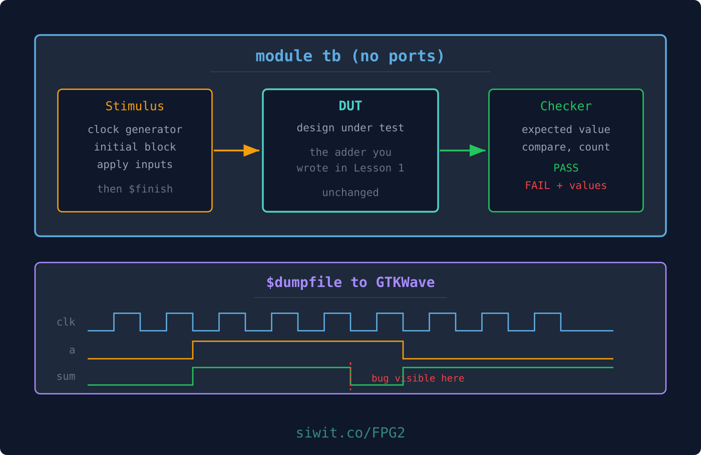
A testbench is an ordinary Verilog module with one unusual property: it has no ports. Nothing drives it, because it sits at the top of the hierarchy. Its job is to instantiate the thing being tested, drive its inputs, and watch its outputs.

The design being tested is called the DUT (design under test) or UUT (unit under test). Both names are in common use.

Every testbench has the same five parts:

1. Declare the testbench module, with an empty port list.

2. Declare signals to connect to the DUT. Anything you drive is a reg, anything you observe is a wire.

3. Instantiate the DUT and connect your signals to its ports.

4. Apply stimulus in an initial block, generating a clock if the design needs one.

5. Check the results, ideally by comparing against expected values rather than reading them.

Here is that skeleton:

`timescale 1ns/1ps

module tb_skeleton;

    // Signals: reg for inputs you drive, wire for outputs you watch
    reg  a, b;
    wire y;

    // Instantiate the design under test
    my_design dut (
        .a(a),
        .b(b),
        .y(y)
    );

    // Stimulus
    initial begin
        a = 0; b = 0;
        #10 a = 1;
        #10 b = 1;
        #10 $finish;
    end

endmodule

The timescale directive

`timescale 1ns/1ps

This says a bare 1 in a delay means one nanosecond, and timing rounds to picoseconds. Without it, the meaning of #10 is left to the simulator and your delays stop being portable. Put it at the top of every testbench.

Delays and ending a simulation

#10 means “wait ten time units.” It exists only in simulation, because no gate waits. The same applies to $finish, $display, $monitor and $dumpfile: anything with a $ is a command to the simulator, not a description of hardware.

$finish matters more than it looks. Without it, a testbench with a running clock never ends and your simulation spins until you kill it.

Generating Stimulus

A clock

Any sequential design needs one. The idiom is a forever loop with a half-period delay:

reg clk;

initial begin
    clk = 0;
    forever #5 clk = ~clk;   // toggles every 5ns, so a 10ns period, 100 MHz
end

Note that it is a half period. A full cycle takes two toggles, so #5 gives 10 ns, not 5 ns. Getting this backwards is common and confusing, because everything still works, just at half the frequency you intended.

Reset, then data

Sequential designs must start from a known state. Assert reset, hold it across at least one clock edge, then release:

initial begin
    reset = 1;
    #20;            // hold through two clock edges at 10ns period
    reset = 0;
end

Walking through input combinations

For combinational logic with few inputs, test all of them. An array of test vectors reads clearly and extends easily:

`timescale 1ns/1ps
`include "first_system.v"

module first_system_tb;

// Inputs
reg in1t, in2t;

// Outputs
wire out1t, out2t;

// Instantiate the Unit Under Test (UUT)
first_system UUT (
    .out1(out1t),
    .out2(out2t),
    .in1(in1t),
    .in2(in2t)
);

reg [1:0] Testset [3:0];

integer count;

// Providing input to the UUT
initial begin
    // Create VCD file for waveform viewing
    $dumpfile("first_system.vcd");
    $dumpvars(0, first_system_tb);

    // Initialize test vectors
    Testset[0] = 2'b00;
    Testset[1] = 2'b01;
    Testset[2] = 2'b10;
    Testset[3] = 2'b11;

    #100;

    count = 0;
    repeat (4)
    begin
        #50 {in1t, in2t} = Testset[count];
        #50 count = count + 1;
    end

    #50 $finish;
end

// Display the result on the console (optional)
initial begin
    $display("================================");
    $display("  in1  in2  |  out1  out2");
    $display("================================");
    $monitor("  %b    %b    |   %b     %b", in1t, in2t, out1t, out2t);
end

endmodule

Two constructs worth naming. reg [1:0] Testset [3:0] declares an array of four two-bit values, which is memory in simulation and needs no hardware. And {in1t, in2t} = Testset[count] uses the concatenation operator {} to assign both signals from one two-bit value at once.

Running it against the first_system module from Lesson 1 gives:

Printing values: display versus monitor

$display prints once, when execution reaches it. $monitor is armed once and then prints automatically whenever any of its arguments changes. One $monitor over the interesting signals often replaces a dozen $display calls.

Useful format specifiers: %b binary, %d decimal, %h hex, %0t simulation time, %s string. The 0 in %0d and %0t drops the padding, which makes output far easier to read.

Self-Checking with Assertions

Everything so far prints a table for a human. That does not scale. Four combinations you can check by eye, sixteen you will skim, two hundred you will not read at all, which means a regression walks straight past you.

A self-checking testbench computes the answer itself and compares:

`timescale 1ns/1ps

module adder4_tb;

    reg  [3:0] a, b;
    reg        cin;
    wire [3:0] sum;
    wire       cout;

    integer i, j;
    integer errors;
    reg [4:0] expected;      // 5 bits: four sum bits plus carry out

    adder4 dut (
        .a(a), .b(b), .cin(cin),
        .sum(sum), .cout(cout)
    );

    initial begin
        $dumpfile("adder4.vcd");
        $dumpvars(0, adder4_tb);

        errors = 0;
        cin    = 0;

        // Exhaustive over both 4-bit inputs: 256 combinations
        for (i = 0; i < 16; i = i + 1) begin
            for (j = 0; j < 16; j = j + 1) begin
                a = i[3:0];
                b = j[3:0];
                #5;                          // let the logic settle

                expected = i + j;            // independent reference answer

                if ({cout, sum} !== expected) begin
                    errors = errors + 1;
                    $display("FAIL  a=%0d b=%0d  got %0d  expected %0d",
                             a, b, {cout, sum}, expected);
                end
            end
        end

        if (errors == 0)
            $display("PASS  all 256 combinations correct");
        else
            $display("FAIL  %0d of 256 combinations wrong", errors);

        $finish;
    end

endmodule

Run it and you get a single line:

PASS  all 256 combinations correct

That is the shape to reach for. Every case tested, one line of verdict, and on failure it names the exact inputs that broke it.

Three details that matter more than they look:

• !== rather than !=. The four-state comparison also catches x (unknown) and z (high impedance). Plain != returns x when either side is unknown, and x is not true, so the else branch runs and your test reports success on a completely undriven output. Use !== in testbenches.
• The reference is independent. expected = i + j uses the simulator’s own arithmetic, not your adder. A reference model that shares logic with the design shares its bugs.
• #5 before checking. Combinational output needs simulation time to settle after inputs change. Check too early and you read the previous value.

Checking a sequential design

For the counter, the property worth testing is that it advances by exactly one per clock edge and wraps cleanly:

`timescale 1ns/1ps

module counter_4bit_tb;

    reg clk;
    reg reset;
    wire [3:0] count;

    reg [3:0] expected;
    integer   errors;

    counter_4bit uut (
        .clk(clk),
        .reset(reset),
        .count(count)
    );

    // Clock generation: 10ns period
    initial begin
        clk = 0;
        forever #5 clk = ~clk;
    end

    initial begin
        $dumpfile("counter_4bit.vcd");
        $dumpvars(0, counter_4bit_tb);

        errors  = 0;
        reset   = 1;
        #20;
        reset    = 0;
        expected = 0;

        // 20 edges, which carries it past the wrap at 15
        repeat (20) begin
            @(posedge clk);
            #1;                          // settle after the edge
            expected = expected + 1;
            if (count !== expected) begin
                errors = errors + 1;
                $display("FAIL  t=%0t  got %0d  expected %0d",
                         $time, count, expected);
            end
        end

        if (errors == 0) $display("PASS  counter advanced correctly through wrap");
        else             $display("FAIL  %0d mismatches", errors);

        $finish;
    end

endmodule

@(posedge clk) is an event control: it pauses until the next rising edge. It is far more robust than counting delays by hand, because it stays correct when you change the clock period.

The #1 after the edge matters. At the exact instant of an edge, whether you observe the old or new value of count is a race. Waiting a nanosecond puts you safely after the flip-flop has settled.

Note that expected is only four bits wide, so it wraps at 15 exactly as the counter does. That is deliberate: the test confirms the wrap rather than flagging it as an error.

Dumping and Reading Waveforms

A pass or fail line tells you that something broke. A waveform tells you why.

initial begin
    $dumpfile("design.vcd");     // the output file
    $dumpvars(0, tb_module);     // 0 means all levels below tb_module
end

$dumpvars(0, tb_module) records everything, including signals inside the DUT, which is what you want while debugging. A smaller depth records less, and only matters on large designs where VCD files grow quickly.

Then run the loop:

iverilog -o counter_4bit_tb.vvp counter_4bit_tb.v counter_4bit.v
vvp counter_4bit_tb.vvp
gtkwave counter_4bit.vcd

Note that both files are listed. Icarus needs the design as well as the testbench. The alternative is an `include "counter_4bit.v" line at the top of the testbench, as in first_system_tb.v above. Pick one convention and stay with it, because doing both gives you duplicate module definitions and a confusing error.

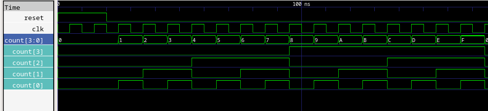
Figure: the counter advancing one step per clock edge, viewed in GTKWave

Reading a trace

In GTKWave, drag signals from the hierarchy pane into the wave pane. A few habits make traces far easier to read:

• Put the clock at the top. Everything is measured against it.
• Put reset next. Most confusing early traces turn out to be reset behaving differently from how you assumed.
• Group buses and display them in hex or decimal rather than as loose bits.
• Read edge by edge. At each rising edge, ask what the inputs to a flip-flop were just before the edge. That, not the value after, determined the new state.

That last habit is the whole skill. Sequential bugs are almost always a signal arriving one cycle later, or earlier, than you assumed.

Application Questions and Solutions

Question 1: Why did the sum look correct but the carry was wrong?

A learner reports that their adder testbench shows the correct sum but cout is always zero. The waveform shows cout flat across every input. What is the likely cause and how would you confirm it?

Question 2: Why does this testbench report success on a broken design?

initial begin
    a = 4'd3; b = 4'd4;
    if (sum != 4'd7) $display("FAIL");
    else             $display("PASS");
    $finish;
end

Give three separate reasons this test cannot be trusted.

Question 3: The design simulates perfectly and fails on the board

A design passes every test. On the FPGA it does not work at all. The clocked block looks like this:

always @(posedge clk) begin
    #5 count <= count + 1;
end

What is wrong?

Summary

You can now prove a design correct before it exists physically, which is the discipline that makes everything after this affordable. Next you apply it to the most important sequential building block there is.