



Mechanical advantage
The force ratio is the reciprocal of the velocity ratio. Motion and force are two views of one machine.
このコンテンツはまだ日本語訳がありません。
Five lessons told you how a mechanism moves. This one tells you what it costs in force, and how to design for it. A toggle clamp turns a light hand pull into a heavy clamping force; a scissor lift needs a hydraulic cylinder whose force runs away as the platform nears the floor; every pin and link must carry its load without breaking. Force analysis is statics done on the mechanism in a chosen position: free-body diagrams and force polygons give the joint reactions, the transmission angle warns where the force transmits badly, and stress sizing turns those forces into metal. The course then closes by running the whole process backward, synthesis: choosing a mechanism and its dimensions to meet a target. #ForceAnalysis #TransmissionAngle #MechanismSynthesis
By the end of this lesson, you will be able to:
A toggle clamp on a machining fixture must hold a part down with several hundred newtons, applied by hand and held without effort while the tool cuts. The designer must answer: what hand force gives the required clamping force, what loads do the pins and links then carry, and are they strong enough? The same questions decide the hydraulic cylinder on a scissor lift and the motor on an engine. Motion analysis found the speeds and accelerations; now we find the forces they imply and the sizes they demand.
Engineering Question: For a given input force or torque, what force appears at the output, what reactions load each joint, and are the links and pins strong enough?
Mechanical advantage
The force ratio is the reciprocal of the velocity ratio. Motion and force are two views of one machine.
Joint reactions
Free-body diagrams and force polygons give the pin loads that bearings and links must carry.
Transmission angle
It measures how much of the joint force does useful work. Near the bad zones a mechanism wastes force and wears.
Synthesis
Run the analysis backward to choose a mechanism type and its link lengths so the target is met.
The Force Polygon
A link in static equilibrium has forces that sum to zero, so drawn tip to tail they close into a polygon. Two special cases do most of the work:
The force polygon is the statics counterpart of the velocity and acceleration polygons: the same draw-to-scale-and-measure method, now for forces.
Force Ratio is the Reciprocal of the Velocity Ratio
An ideal (lossless) mechanism conserves power: input power equals output power. With
The mechanical advantage is the reciprocal of the velocity ratio found in the velocity analysis. Where the output slows (a limit or toggle position, velocity ratio toward zero), the mechanical advantage grows large. This is why the same toggle position that stopped the output in the velocity analysis amplifies force here. Real mechanisms lose a little to friction, so an efficiency
Transmission Angle and Allowable Stress
The transmission angle
Once a joint force
The pin, in shear. The pin is cut across its section by the joint force:
Count the shear planes before anything else. A pin in a simple lap joint is cut on one plane; a pin in a clevis or fork, supported on both sides, is cut on two, which halves the stress for the same force. Most linkage pins are in double shear, so assuming single shear is the safe, conservative choice when a question does not say.
The link, in bending. A rectangular link of thickness
Note that
This is the capstone worked example: from hand force to clamping force by force polygon, then the pin and link stresses. The force polygon is the same graphical method used for velocities and accelerations, now applied to forces: draw the balance to scale, solve it exactly, and confirm in the simulator.
Simulator and hands-on lab
Hands-on lab: Continue in the Toggle Clamp Experiments lab (siwit.co/TCM). Experiments 2 and 4 cover force amplification and pin/link stress sizing.
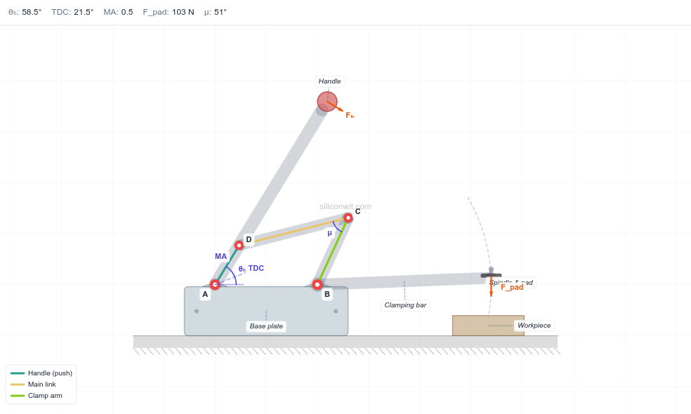
The main link is a two-force member, so its force is along the link. The clamp arm is a three-force member (pad reaction, main-link force, pivot reaction), so its force triangle closes.
Identify the members. The main link carries a force along its own line (two-force member). The clamp arm then has three forces: the main-link push at one joint, the pad reaction at the workpiece, and the pivot reaction at
Draw the triangle. Choose a force scale and mark it (for example 1 cm = 20 N). Lay the known main-link force tip to tail with the pad-reaction direction; the pivot reaction closes the triangle. Measuring the sides gives the pad force and the pivot force. ✅
The over-centre amplification. Geometrically the ideal force ratio of the toggle is

Mechanical advantage at the
taking it in two stages,
Clamping force:
The closer the rest position is set to top-dead-centre, the higher this rises, the over-centre design from Lessons 1 and 3 seen as force.
Pin shear at a representative link/pin force of
Pin safety factor, against the shear yield, not the tensile yield:
Had the pin been in double shear the stress would halve to
Link bending stress, with
The same result through
Link safety factor and the verdict:
Both parts clear the required
Open the simulator (siwit.co/TCM) and set the hand force, lock margin, efficiency, and the pin and link sizes. ✅
Confirm the clamping force rises sharply as the lock margin shrinks toward centre, and read the pin-shear and link-bending stresses with their pass/fail verdict against the allowable. They match the hand calculation. ✅
The transmission angle tells you where in its cycle a four-bar transmits force well, and where it wastes it.
Simulator and hands-on lab
Hands-on lab: Continue in the Four-Bar Linkage Experiments lab (siwit.co/FBL). Experiment 2 maps the transmission angle and mechanism quality.
Measure
Sweep the crank. Across a full turn
Design response. If those zones fall inside the working stroke, change the link lengths (Application 4 synthesis) or re-time the load so the heavy work happens where
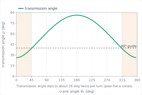
An angle on a chart is not yet an engineering answer. The coupler is a two-force member, so it pushes on the follower along its own line; only the component across the follower does useful work.
Split the coupler force at the joint. With coupler force
The output torque is
Price the good instant and the bad one. At
Rather more than twice the coupler force, and with it rather more than twice the pin and link stresses of Application 1, for no extra useful work. ✅
Note where the rest of it goes. At
Read the guide as a force statement. The
Set it up. Open the simulator (siwit.co/FBL) and set
Match the two readouts. The panel reports Min µ and Max µ directly: ✅
Locate the poor-force zones on the axis. The trace crosses the
Cross-check against mechanical advantage. The Minimum MA should bottom out at exactly the crank angles where
The scissor lift shows mechanical advantage working against the designer: the actuator force runs away as the platform nears the floor.
Simulator and hands-on lab
Hands-on lab: Continue in the Scissor Lift Experiments lab (siwit.co/SLM). Experiment 1 plots the actuator force and Experiment 8 the link stress.
Virtual work is quick, but only once you know which two lengths change and how. Both come off the space diagram, so draw it before writing anything down.
Draw the lift to scale at the angle of interest, say
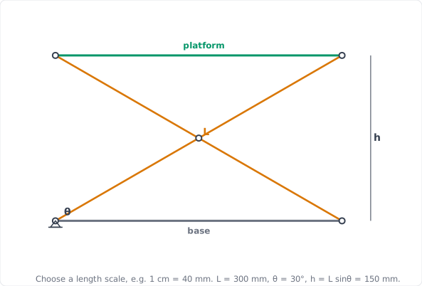
Mark the two lengths that change. The platform height and the base spread the actuator works across: ✅
Note that they move in opposite senses. Raising the platform (
Differentiate both lengths with respect to the scissor angle, giving the virtual displacements for a small rotation
Equate the work. Over a frictionless virtual displacement the actuator’s work equals the work done lifting the load. The actuator shortens
Cancel and read the result. Both
This is for an actuator mounted horizontally across the base. A diagonal or pantograph placement changes the geometry factor, and the simulator reports the value for each type. ✅
Read the runaway. At
Design response. This is why scissor lifts work over a limited low-angle band, use a diagonal or pantograph actuator placement to improve the low-angle advantage, and never start fully flat. ✅
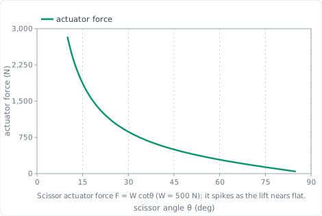
Set it up and read three points off the trace. Open the simulator (siwit.co/SLM), set the platform load to
| Scissor angle | Trace reads | |
|---|---|---|
The
Watch Max Actuator Force follow the lowest angle. The panel’s Max Actuator Force is not a property of the lift; it is whatever the force reaches at the bottom of the stroke you allow. Raise the minimum height and it falls immediately, which is the cheapest design fix available here. ✅
Change the actuator placement. Switch the actuator type to Diagonal Base and watch the low-angle end of the curve drop: the geometry factor has changed, so
Check the link stress. With the actuator force known, the arm stress follows as in Application 1. The lowest angles are the worst case for both force and stress at once, which is why a lift is rated from its lowest working height. ✅
Analysis takes a mechanism and finds its behaviour. Synthesis takes a required behaviour and finds the mechanism. This is where the whole course is put to use.
Simulator and hands-on lab
Hands-on lab: Use the Four-Bar Linkage Experiments lab (siwit.co/FBL) to test each candidate set of link lengths against the target.
Read the family off the task. A continuous input turning an oscillating output points to a crank-rocker four-bar; a straight-line output would point to a slider-crank; a clamping action would point to a toggle. ✅
Confirm one input drives it. The mobility check gives one degree of freedom for a four-bar, so a single motor on the crank fully determines the motion. ✅
The construction rests on one fact from the position analysis: at a limit position the crank and coupler fall into one straight line. Folded, the distance from
Set out the frame. Choose and mark a length scale, say 1 cm = 20 mm. Draw the ground
Draw the rocker at both extremes. Swing the rocker
Measure the two distances from the crank centre to each rocker extreme: ✅
Solve the pair. Adding and subtracting the two measurements separates the unknowns: ✅
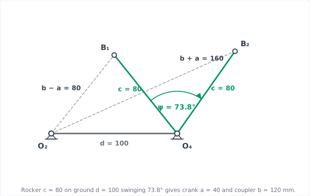
A set of link lengths that meets the motion is only a candidate. It has to survive every analysis in this course before it is a design.
Grashof, so the crank can actually turn all the way round. Shortest plus longest against the other two:
Swing, to confirm the construction did its job. Running the position analysis over a full turn gives a rocker oscillation of
Transmission angle, and here it fails. These are the very link lengths analysed in Application 2, where
This is the ordinary outcome of a first synthesis, not a mistake in the construction. The limit-position method controls the motion and says nothing whatever about force quality. ✅
Identify what is actually free. The ground
Shorten the rocker and re-place the swing. Repeating Step 2 with
Re-run every check. Grashof still passes (
The linkage no longer drops below the guide at any point in the cycle, against
Recognise the loop. Nothing here was solved in one pass. Synthesis is propose, analyse, refine, repeated until every check clears, and the analysis tools of the previous five lessons are precisely the tests being run. ✅
Check the swing without trusting your drawing. Enter the refined lengths in the simulator (siwit.co/FBL) and read the Oscillation result: it reports the rocker’s total swing directly, and should show about
Compare both candidates side by side. Put in
Run the full sequence on the survivor. Mobility, position, velocity and mechanical advantage, acceleration and inertia loads, then joint forces and pin and link stresses as in Application 1. A design is finished only when all of them pass. ✅
Take it to CAD. The surviving link lengths and limit positions become the sketch constraints of a real part in the Parametric Mechanical CAD with FreeCAD course. ✅
Spot the two-force members
A link loaded at only two joints carries force along its line. Finding these first collapses most of the force polygon.
Force is the reciprocal of motion
Use the velocity ratio: mechanical advantage is its reciprocal. No separate force derivation is needed for the ideal value.
Keep the transmission angle up
Hold
Synthesis is analysis in a loop
Propose dimensions, run every analysis as a test, refine, and repeat until all checks pass.
| Mechanism | What you solve for | Key relation | Simulator |
|---|---|---|---|
| Toggle clamp | clamping force, stresses | siwit.co/TCM | |
| Four-bar | transmission angle | siwit.co/FBL | |
| Scissor lift | actuator force | siwit.co/SLM | |
| Crank-slider | crank torque | siwit.co/CSM |
| Step | Relation |
|---|---|
| Pin shear stress | |
| Shear yield | |
| Link bending stress | |
| Safety factors | |
| Verdict | both must exceed the required |
You met four mechanisms and analysed each through six lenses: whether it moves, where its links sit, how fast they move, how hard they accelerate and what inertia that creates, how to program a motion with a cam, and what forces flow through it and how to design for them. Every result was drawn to scale by hand, confirmed by calculation, and checked in an interactive simulator. That triad, the drawing for intuition, the mathematics for precision, and the simulator for exploration, is how planar mechanisms are understood and designed.
The force polygons, transmission-angle and actuator-force curves here were drawn from the statics and reproduced with a few lines of Python (NumPy). The simulators confirm the forces and report the stress verdicts. No specialised software is required; statics on a mechanism is the whole method.
Comments